Moving Average#
Introduction#
In this section, we will build upon that knowledge and explore another important concept called smoothing.
In particular, we will cover:
An introduction to smoothing and why it is necessary.
Common smoothing techniques.
How to smooth time series data with Python and generate forecasts.
Smoothing#
A data collection process is often affected by noise.
If too strong, the noise can conceal useful patterns in the data.
Smoothing is a well-known and often-used technique to recover those patterns by filtering out noise.
It can also be used to make forecasts by projecting the recovered patterns into the future.
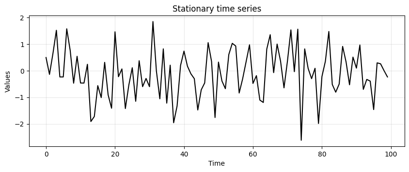
We start by generating some stationary data.
We discussed the importance of visually inspecting the time series with a run-sequence plot.
So, we will also define the
run_sequence_plotfunction to visualize our data.
# Generate stationary data
time = np.arange(100)
stationary = np.random.normal(loc=0, scale=1.0, size=len(time))
run_sequence_plot(time, stationary, title="Stationary time series");
Simple smoothing techniques#
There are many techniques for smoothing data.
The most simple ones are:
Simple average
Moving average
Weighted moving average
Simple average#
Simple average is the most basic technique.
Consider the stationary data above.
The most conservative way to represent it is through its mean.
The mean can be used to predict the future values of the time series.
This type of representation is called simple average.
# find mean of series
stationary_time_series_avg = np.mean(stationary)

# create array composed of mean value and equal to length of time array
sts_avg = np.full(shape=len(time), fill_value=stationary_time_series_avg, dtype='float')
ax = run_sequence_plot(time, stationary, title="Stationary Data")
ax.plot(time, sts_avg, 'tab:red', label="mean")
plt.legend();
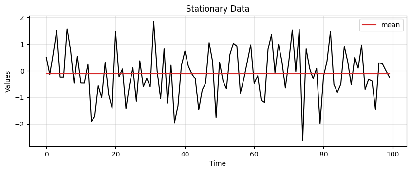
Exceptional! But we can do better…
Mean squared error (MSE)#
The approximation with the mean seems reasonable in this case.
In general we want to measure how far off our estimate is from reality.
A common way of doing it is by calculating the Mean Squared Error (MSE)
where \(X(t)\) and \(\hat{X}(t)\) are the true and estimated values at time \(t\), respectively.
def mse(observations, estimates):

    # check length of arrays equal
    assert len(observations) == len(estimates), "Arrays must be of equal length"

    # calculations
    difference = observations - estimates
    sq_diff = difference ** 2
    mse = np.mean(sq_diff)

    return mse
y_true = np.array([2, 3, 1, 4, 3, 5, 4, 6, 5, 7])
y_pred = np.array([2.5, 1.0, 3.5, 3.8, 6.0, 4.5, 5.5, 4.0, 6.5, 7.5])

zeros = mse(y_true, y_pred)
print(zeros)
2.854
Next, we add a trend to our stationary time series.
trend = (time * 2.0) + stationary
run_sequence_plot(time, trend, title="Time series with trend");
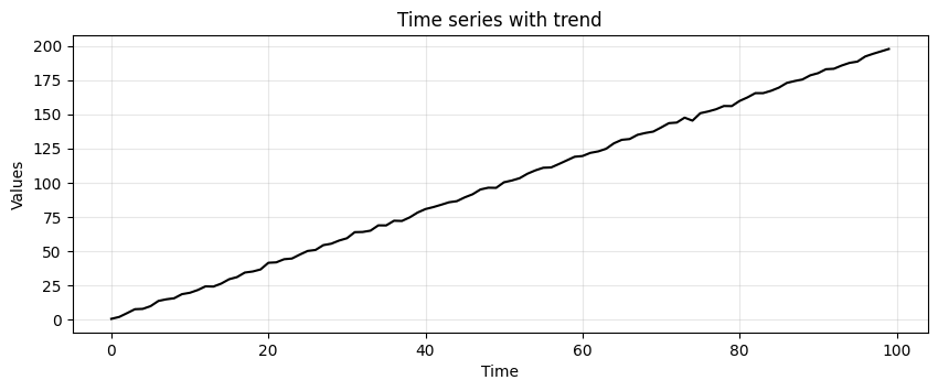
Let’s try our simple average again!
# find mean of series
trend_time_series_avg = np.mean(trend)

# create array of mean value equal to length of time array
avg_trend = np.full(shape=len(time), fill_value=trend_time_series_avg, dtype='float')

run_sequence_plot(time, trend, title="Time series with trend")
plt.plot(time, avg_trend, 'tab:red', label="mean")
plt.legend();
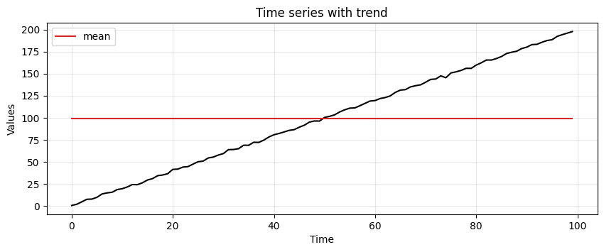
We must find other ways to capture the underlying pattern in the data.
We start with something called a moving average.
Moving Average (MA)#
Moving average has a greater sensitivity than the simple average to local changes in the data.
The easiest way to understand moving average is by example.
The first step is to select a window size.
We’ll arbitrarily choose a size of 3.
Then, we start computing the average for the first three values and store the result.
We then slide the window by one and calculate the average of the next three values.
We repeat this process until we reach the final observed value.
Now, let’s define a function to perform smoothing with the MA.
Then, we compare the MSE obtained from applying simple and moving average on the data with trend.
def moving_average(observations, window=3, forecast=False):
    cumulative_sum = np.cumsum(observations, dtype=float)
    cumulative_sum[window:] = cumulative_sum[window:] - cumulative_sum[:-window]
    ma = cumulative_sum[window - 1:] / window
    if forecast:
        observations = np.append(observations, np.nan)
        ma_forecast = np.insert(ma, 0, np.nan*np.ones(window))
        return observations, ma_forecast
    else:
        return ma
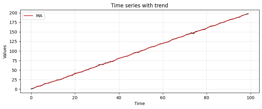
MA_trend = moving_average(trend, window=3)

print(f"MSE:\n--------\nsimple average: {mse(trend, avg_trend):.2f}\nmoving_average: {mse(trend[2:], MA_trend):.2f}")
MSE:
--------
simple average: 3338.46
moving_average: 4.56
We can tell that the MA manages to pick up the trend much better
Let’s plot the moving average to see what it is doing
run_sequence_plot(time, trend, title="Time series with trend")
plt.plot(time[1:-1], MA_trend, 'tab:red', label="MA")
plt.legend();
Let’s up the ante, we’ll introduce some seasonality
seasonality = 10 + np.sin(time) * 10 + stationary
MA_seasonality = moving_average(seasonality, window=3)
run_sequence_plot(time, seasonality, title="Seasonality")
plt.plot(time[1:-1], MA_seasonality, 'tab:red', label="MA")
plt.legend(loc='upper left');
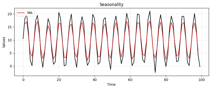
It’s not perfect but clearly picks up the periodic pattern.
Lastly, let’s see how MA handles trend, seasonality, and a bit of noise.
trend_seasonality = trend + seasonality + stationary
MA_trend_seasonality = moving_average(trend_seasonality, window=3)
run_sequence_plot(time, trend_seasonality, title="Trend, seasonality, and noise")
plt.plot(time[1:-1], MA_trend_seasonality, 'tab:red', label="MA")
plt.legend(loc='upper left');
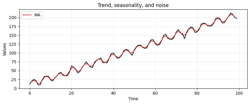
This method is picking up key patterns in these toy datasets.
However, it has several limitations.
MA assigns equal importance to all values in the window, regardless of their chronological order.
For this reason it fails in capturing the often more relevant recent trends.
MA requires the selection of a specific window size, which can be arbitrary and may not suit all types of data.
a small window may lead to noise
a too large window could oversmooth the data, missing important short-term fluctuations.
MA does not adjust for changes in trend or seasonality.
This can lead to inaccurate predictions, especially when these components are nonlinear and time-dependent.
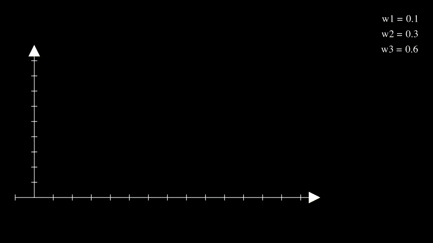
Weighted moving average (WMA)#
WMA weights recent observations more than more distant ones.
This makes intuitive sense.
Think of the stock market: it has been observed that today’s price is a good predictor of tomorrow’s price.
By applying unequal weights to past observations, we can control how much each affects the future forecast.
There are many ways to set the weights and a discussion about this topic is beyond the scope of this workshop (see here)
In the following example, weights of 0.1, 0.3, and 0.6 are used
Forecasting with MA#
Instead of pulling out the inherent pattern within a series, the smoothing functions can be used to create forecasts.
The forecast for the next time step is computed as follows:
where \(P\) is the window size of the MA.
Let’s consider the following time series \(X= [1, 2, 4, 8, 16, 32, 64]\).
In particular, we apply the smoothing process and use the resulting value as forecast for the next time step.
With the MA technique and a window size \(P=3\) we get the following forecast.
x = np.array([1, 2, 4, 8, 16, 32, 64])
ma_x, ma_forecast = moving_average(x, window=3, forecast=True)
t = np.arange(len(ma_x))
run_sequence_plot(t[:-4], ma_x[:-4], title="Nonlinear data")
plt.plot(t[-5:], ma_x[-5:], 'k', label="True values", linestyle='--')
plt.plot(t, ma_forecast, 'tab:red', label="MA forecast", linestyle='--')
plt.legend(loc='upper left');
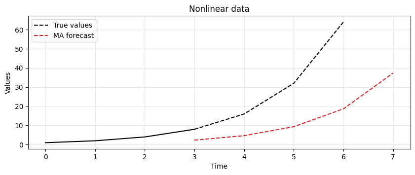
The result shows that MA is lagging behind the actual signal.
In this case, it is not able to keep up with changes in the trend.
The lag of MA is also reflected in the forecasts it produces.
Let’s focus on the forecasting formula we just defined.
While easy to understand, one of its properties may not be obvious.
What’s the lag associated with this technique?
In other words, after how many time steps do we see a local change in the underlying signal?
The answer is: \(\frac{(P+1)}{2}\).
For example, say you’re averaging the past 5 values to make the next prediction.
Then the forecast value that most closely reflects the current value will appear after \(\frac{5+1}{2} = 3\) time steps.
Clearly, the lag increases as you increase the window size for averaging.
One might reduce the window size to obtain a more responsive model.
However, a window size that’s too small will chase noise in the data as opposed to extracting the pattern.
There is a tradeoff between responsiveness and robustness to noise.
The best answer lies somewhere in between and requires careful tuning to determine which setup is best for a given dataset and problem at hand.
Let’s make a practical example to show this tradeoff.
We will generate some toy data and apply a MA with different window sizes.
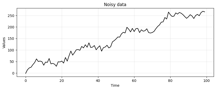
To make things more clear, we generate again data with trend and seasonality, but we add more noise.
noisy_noise = np.random.normal(loc=0, scale=8.0, size=len(time))
noisy_trend = time * 2.75
noisy_seasonality = 10 + np.sin(time * 0.25) * 20
noisy_data = noisy_trend + noisy_seasonality + noisy_noise

run_sequence_plot(time, noisy_data, title="Noisy data");
# Compute MA with different window sizes
lag_2 = moving_average(noisy_data, window=3)
lag_3 = moving_average(noisy_data, window=5)
lag_5 = moving_average(noisy_data, window=9)
lag_10 = moving_average(noisy_data, window=19)
_, axes = plt.subplots(2,2, figsize=(11,6))
axes[0,0] = run_sequence_plot(time, noisy_data, title="MA with lag 2", ax=axes[0,0])
axes[0,0].plot(time[1:-1], lag_2, color='tab:blue', linewidth=2.5)
axes[0,1] = run_sequence_plot(time, noisy_data, title="MA with lag 3", ax=axes[0,1])
axes[0,1].plot(time[2:-2], lag_3, color='tab:orange', linewidth=2.5)
axes[1,0] = run_sequence_plot(time, noisy_data, title="MA with lag 5", ax=axes[1,0])
axes[1,0].plot(time[4:-4], lag_5, color='tab:green', linewidth=2.5)
axes[1,1] = run_sequence_plot(time, noisy_data, title="MA with lag 10", ax=axes[1,1])
axes[1,1].plot(time[9:-9], lag_10, color='tab:red', linewidth=2.5)
plt.tight_layout();
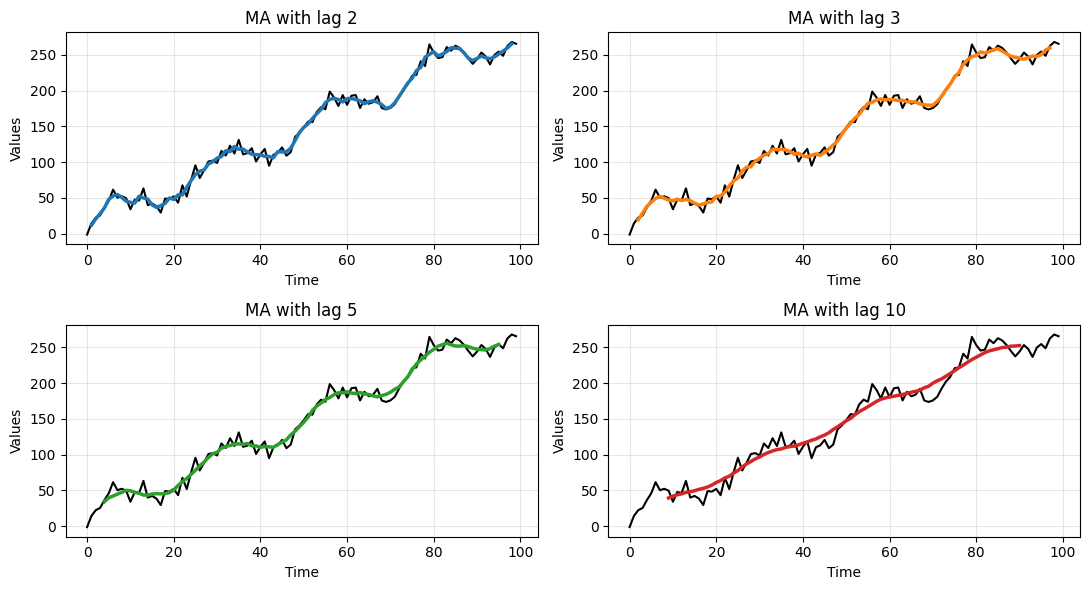
Clearly, the larger the window size the smoother the data.
This allows to get rid of the noise but, eventually, also the underlying signal is smoothed out.
Exponential Smoothing#
There are three key exponential smoothing techniques:
Type |
Capture trend |
Capture seasonality |
|---|---|---|
Single Exponential Smoothing |
❌ |
❌ |
Double Exponential Smoothing |
✅ |
❌ |
Triple Exponential Smoothing |
✅ |
✅ |
We don’t have enough time to go through the math of how it works, but it is analogous to the WMA
The basic formulation is:
where:
\(S(t)\) is the smoothed value at time t,
\(\alpha\) is a smoothing constant,
\(X(t)\) is the value of the series at time t.
Double Exponential Smoothing also has is able to pick up on trend by using an estimated trend.
Triple Exponential Smoothing is able to additionally pick up on seasonality.
Let’s relax off the math, and demonstrate Exponential Smoothing by letting
statsmodelsdo the work for us.
We will holdout the last 5 samples from the dataset (i.e., they become the test set).
We will compare the predictions made by the models with these values.
# Train/test split
train = trend_seasonality[:-5]
test = trend_seasonality[-5:]
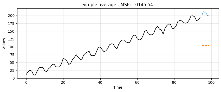
Simple Average#
This is a very crude model to say the least.
It can at least be used as a baseline.
Any model we try moving forward should do much better than this one.
# find mean of series
trend_seasonal_avg = np.mean(train)

# create array of mean value equal to length of time array
simple_avg_preds = np.full(shape=len(test), fill_value=trend_seasonal_avg, dtype='float')

# mse
simple_mse = mse(test, simple_avg_preds)

# results
print("Predictions: ", simple_avg_preds)
print("MSE: ", simple_mse)
Predictions:  [103.69796574 103.69796574 103.69796574 103.69796574 103.69796574]
MSE:  10145.54276901901
ax = run_sequence_plot(time[:-5], train, title=f"Simple average - MSE: {simple_mse:.2f}")
ax.plot(time[-5:], test, color='tab:blue', linestyle="--", label="test")
ax.plot(time[-5:], simple_avg_preds, color='tab:orange', linestyle="--", label="preds");
Single Exponential#
from statsmodels.tsa.api import SimpleExpSmoothing

single = SimpleExpSmoothing(train).fit(optimized=True)
single_preds = single.forecast(len(test))
single_mse = mse(test, single_preds)
print("Predictions: ", single_preds)
print("MSE: ", single_mse)
Predictions:  [194.37115555 194.37115555 194.37115555 194.37115555 194.37115555]
MSE:  129.47602005761325
ax = run_sequence_plot(time[:-5], train, title=f"Simple exponential smoothing - MSE: {single_mse:.2f}")
ax.plot(time[-5:], test, color='tab:blue', linestyle="--", label="test")
ax.plot(time[-5:], single_preds, color='tab:orange', linestyle="--", label="preds");
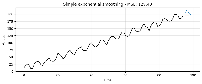
Although better than the simple average method, it’s still pretty crude.
Notice how the forecast is just a horizontal line.
Single Exponential Smoothing cannot pick up neither trend nor seasonality.
Double Exponential#
from statsmodels.tsa.api import Holt

double = Holt(train).fit(optimized=True)
double_preds = double.forecast(len(test))
double_mse = mse(test, double_preds)
print("Predictions: ", double_preds)
print("MSE: ", double_mse)
Predictions:  [196.20305952 198.03496347 199.86686742 201.69877137 203.53067532]
MSE:  74.27670577417757
ax = run_sequence_plot(time[:-5], train, title=f"Double exponential smoothing - MSE: {double_mse:.2f}")
ax.plot(time[-5:], test, color='tab:blue', linestyle="--", label="test")
ax.plot(time[-5:], double_preds, color='tab:orange', linestyle="--", label="preds");
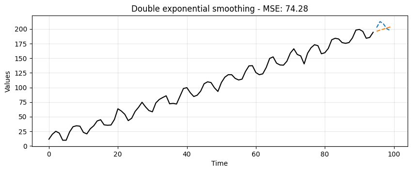
Double Exponential Smoothing can pickup on trend, which is exactly what we see here.
This is a significant leap but no quite yet the prediction we would like to get.
from statsmodels.tsa.api import ExponentialSmoothing

triple = ExponentialSmoothing(train,
                              trend="additive",
                              seasonal="additive",
                              seasonal_periods=13).fit(optimized=True)
triple_preds = triple.forecast(len(test))
triple_mse = mse(test, triple_preds)
print("Predictions: ", triple_preds)
print("MSE: ", triple_mse)
Predictions:  [207.46349451 210.02635851 208.80394709 202.63149745 201.40914672]
MSE:  10.983389218197164
ax = run_sequence_plot(time[:-5], train, title=f"Triple exponential smoothing - MSE: {triple_mse:.2f}")
ax.plot(time[-5:], test, color='tab:blue', linestyle="--", label="test")
ax.plot(time[-5:], triple_preds, color='tab:orange', linestyle="--", label="preds");
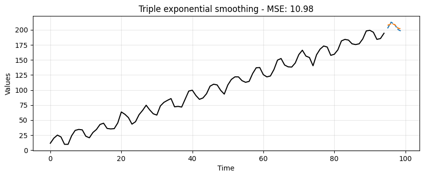
Triple Exponential Smoothing picks up trend and seasonality.
Clearly, this is the most suitable approach for this data.
We can summarize the results in the following table:
data_dict = {'MSE':[simple_mse, single_mse, double_mse, triple_mse]}
df = pd.DataFrame(data_dict, index=['simple', 'single', 'double', 'triple'])
print(df)
                 MSE
simple  10145.542769
single    129.476020
double     74.276706
triple     10.983389
Summary#
In this lecture we learned
What is smoothing and why it is necessary.
Some common smoothing techniques.
A basic understanding of how to smooth time series data with Python and generate forecasts.
Exercise: Try it yourself! Pick any stock and use the first, second, and third order EMA to forecast the values.
def forecast_stock(ticker, start=None, end=None, test_size=5, plot=True):

    # Download stock data
    data = yf.download(ticker, start=start, end=end)
    series = data['Close'].dropna().values
    time = np.arange(len(series))

    # Train/test split
    train = series[:-test_size]
    test = series[-test_size:]

    # Estimate seasonal period using FFT
    def estimate_seasonal_period(y):
        y = np.array(y)
        y_centered = y - np.mean(y)
        fft_vals = np.fft.fft(y_centered)
        fft_mag = np.abs(fft_vals)[:len(y)//2]
        freqs = np.fft.fftfreq(len(y), d=1)[:len(y)//2]
        fft_mag[0] = 0
        dominant_freq = freqs[np.argmax(fft_mag)]
        return max(1, int(round(1 / dominant_freq)))

    seasonal_period = estimate_seasonal_period(train)
    print(f"Estimated seasonal period: {seasonal_period}")

    results = {}

    # Simple Exponential Smoothing
    ses_model = SimpleExpSmoothing(train).fit(optimized=True)
    ses_preds = ses_model.forecast(len(test))
    ses_mse = mse(test, ses_preds)
    results['SES'] = {'preds': ses_preds, 'mse': ses_mse}

    # Holt's Linear Trend
    holt_model = Holt(train).fit(optimized=True)
    holt_preds = holt_model.forecast(len(test))
    holt_mse = mse(test, holt_preds)
    results['Holt'] = {'preds': holt_preds, 'mse': holt_mse}

    # Holt-Winters (Triple Exponential Smoothing)
    hw_model = ExponentialSmoothing(
        train, trend="additive", seasonal="additive",
        seasonal_periods=seasonal_period
    ).fit(optimized=True)
    hw_preds = hw_model.forecast(len(test))
    hw_mse = mse(test, hw_preds)
    results['Holt-Winters'] = {'preds': hw_preds, 'mse': hw_mse}

    # Plotting
    if plot:
        plt.figure(figsize=(12, 5))
        plt.plot(time, series, color='tab:blue', label='Full series')
        plt.plot(time[-test_size:], test, 'b--', label='Test data')
        plt.plot(time[-test_size:], ses_preds, 'orange', linestyle='--', label='First order exponential preds')
        plt.plot(time[-test_size:], holt_preds, 'green', linestyle='--', label='Second order exponential preds')
        plt.plot(time[-test_size:], hw_preds, 'red', linestyle='--', label='Third order exponential preds')
        plt.title("Stock Forecasting")
        plt.legend()
        plt.show()

    return results
results = forecast_stock("AAPL", start="2023-08-20", end="2025-08-20", test_size=5)
for method, res in results.items():
    print(f"{method} MSE: {res['mse']:.2f}")
    print(f"{method} Predictions: {res['preds']}")
[*********************100%***********************] 1 of 1 completed
Estimated seasonal period: 3
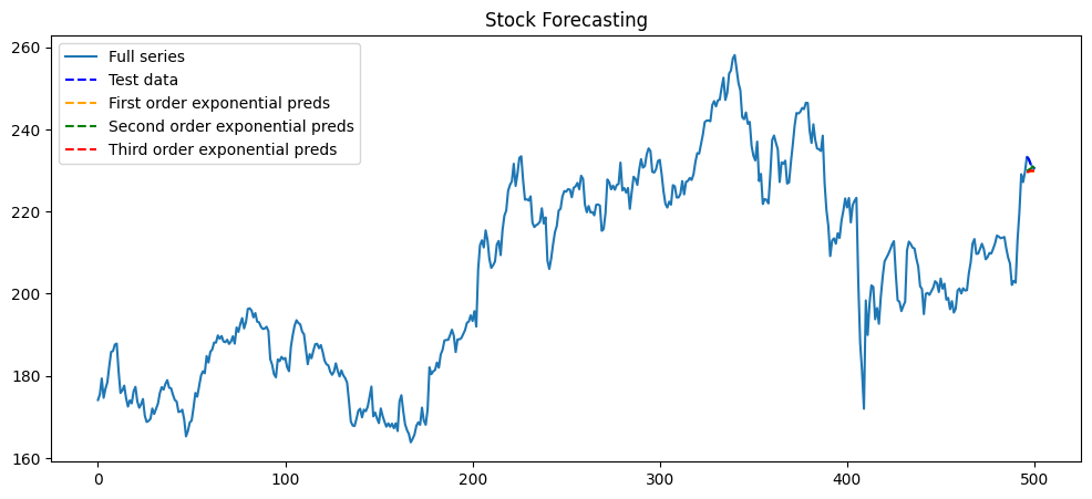
SES MSE: 5.89
SES Predictions: [229.64999386 229.64999386 229.64999386 229.64999386 229.64999386]
Holt MSE: 3.98
Holt Predictions: [229.91659843 230.183203   230.44980756 230.71641213 230.9830167 ]
Holt-Winters MSE: 5.50
Holt-Winters Predictions: [229.57441512 229.68638922 229.98644734 229.9108686  230.0228427 ]