Introduction to Time Series Analysis

Introduction

In this section we will cover the following topics:

• What is a time series, and when do we use it.

• The main components of a time series.

• Time series decomposition.

Show code cell source

Hide code cell source

import numpy as np
import matplotlib.pyplot as plt
import statsmodels.api as sm
import yfinance as yf
import pandas as pd
from statsmodels.tsa.seasonal import seasonal_decompose, STL
from scipy.fft import fft
np.random.seed(42)  # for reproducibility

What is a time series?

• A time series is a sequence of data points organized in time order.

• Usually, the time signal is sampled at equally spaced points in time.

• These can be represented as the sequence of the sampled values.

• We refer to this setting as discrete time.

What data are represented as time series?

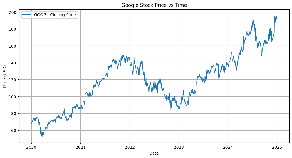
• Time series have a plethora of applications such as modeling finance, activity, behaviour, and so on.

Show code cell source

Hide code cell source

data = yf.download("GOOGL", start="2020-01-01", end="2025-01-01", auto_adjust=True)

plt.figure(figsize=(12, 6))
plt.plot(data.index, data['Close'], label="GOOGL Closing Price")
plt.title("Google Stock Price vs Time")
plt.xlabel("Date")
plt.ylabel("Price (USD)")
plt.legend()
plt.grid(True)
plt.show()

[*********************100%***********************]  1 of 1 completed

Show code cell source

Hide code cell source

data = sm.datasets.get_rdataset("LakeHuron", "datasets")
lake_huron = data.data['value']
years = data.data['time']

plt.figure(figsize=(10, 6))
plt.plot(years, lake_huron, color='steelblue', linewidth=1.5)
plt.title('Lake Huron Water Level (1875-1972)', fontsize=14)
plt.xlabel('Year')
plt.ylabel('Elevation (feet)')
plt.grid(alpha=0.3)
plt.show()

Show code cell source

Hide code cell source

import matplotlib.pyplot as plt
import pandas as pd

# Data from Scottish and Irish Census
data = {
    'Year': [1901, 1911, 1921, 1931, 1941, 1951, 1961, 1971, 1981, 1991, 2001, 2011],
    'Scottish_Gaelic_Speakers': [250000, 200000, 158000, 130000, 105000, 95000, 80000, 88000, 82000, 65000, 58000, 57000],
    'Irish_Gaelic_Speakers': [680000, 620000, 580000, 540000, 555000, 570000, 720000, 790000, 1030000, 1420000, 1670000, 1840000]
}

df = pd.DataFrame(data)

plt.figure(figsize=(12, 7))

plt.plot(df['Year'], df['Scottish_Gaelic_Speakers'], 
         marker='o', linewidth=2, label='Scottish Gaelic Speakers')

plt.plot(df['Year'], df['Irish_Gaelic_Speakers'], 
         marker='s', linewidth=2, label='Irish Gaelic Speakers (Gaeilge)')

plt.title('Number of Gaelic Speakers Over Time', fontsize=16)
plt.xlabel('Year', fontsize=12)
plt.ylabel('Number of Speakers', fontsize=12)
plt.grid(True, alpha=0.3)
plt.legend()
plt.xticks(df['Year'])

plt.annotate('Irish language revival efforts', 
             xy=(1981, 1030000), xytext=(1960, 1500000),
             arrowprops=dict(arrowstyle='->', color='blue'),
             fontsize=10)

plt.tight_layout()
plt.show()

Time series analysis

The main objectives of time series analysis are:

1. To find a model that adequately explains the dependence observed in a time series.

2. To predict or forecast future values of the time series based on those we have already observed.

3. To adjust our observed data into a form more suited for answering the question of interest.

Applications

Time series analysis is applied in many real world applications, including

• Economic forecasting

• Stock market analysis

• Demand planning and forecasting

• Anomaly detection

• … And much more

Economic Forecasting

• Time series analysis is used in macroeconomic predictions.

• World Trade Organization does time series forecasting to predict levels of international trade.

• Federal Reserve uses time series forecasts of the economy to set interest rates [source].

Demand forecasting

• Time series analysis is used to predict demand at different levels of granularity.

• Amazon and other e commerce companies use time series modeling to predict demand at a product geography level [source].

• Helps meet customer needs (fast shipping) and reduce inventory waste

Anomaly detection

• Used to detect anomalous behaviors in the underlying system by looking at unusual patterns in the time series.

• Widely used in manufacturing to detect defects and target preventive maintenance

• With new IoT devices, anomaly detection is being used in machinery heavy industries, such as petroleum and gas [source].

Time series components

• A time series is often assumed to be composed of three components:

  • Trend: The trend is the direction of the data.

  • Seasonality: The seasonal component is the part constantly repeats itself in time.

  • Noise: The component that is neither Trend nor Seasonality.

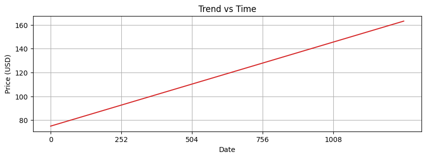
Trend

• Kendall writes that “the essential idea of trend is that it shall be smooth.”

• Trend captures the general direction of the time series.

• Trend can be increasing, decreasing, or constant.

• It can increase/decrease in different ways over time (linearly, exponentially, etc).

• When the trend is removed, we obtain a detrended series.

Show code cell source

Hide code cell source

data = yf.download("GOOGL", start="2020-01-01", end="2025-01-01", auto_adjust=True)

y = data['Close'].dropna().to_numpy().flatten()
x = np.arange(len(y)) 

z = np.polyfit(x, y, 1)
p = np.poly1d(z)

plt.figure(figsize=(12,6))
plt.plot(data.index[:len(y)], y, label="GOOGL Closing Price")
plt.plot(data.index[:len(y)], p(x), "r--", label="Trendline")
plt.title("Google Stock Price with Trendline (2020–2025)")
plt.xlabel("Date")
plt.ylabel("Price (USD)")
plt.legend()
plt.grid(True)
plt.show()

[*********************100%***********************]  1 of 1 completed

• Let’s create a trend from scratch to understand how it’s behaviour.

time = np.arange(252 * 5) # days the market is open * 5
trend = time * 0.07 + 75

Show code cell source

Hide code cell source

fig, ax = plt.subplots(1, 1, figsize=(10, 3))
ax.plot(time, trend, color='tab:red')
ax.set_xlabel("Date")
ax.set_ylabel("Price (USD)")
year_ticks = np.arange(0, len(time), 252)
ax.set_xticks(year_ticks)
ax.grid(True)
plt.title("Trend vs Time");

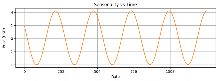
Seasonality

• Periodic fluctuations in time series data that occur at regular intervals due to seasonal factors.

• It is characterized by consistent and predictable patterns over a specific period (e.g., daily, monthly, quarterly, yearly).

• When we remove a seasonal component we say that we deseasonalize the series.

It can be driven by many factors, and there can be multiple causes of seasonal behaviour.

• Naturally occurring events such as weather fluctuations caused by time of year.

• Business or administrative procedures, such as start and end of a school year.

• Social or cultural behavior, e.g., holidays or religious observances.

seasonal = 0.1 + np.sin( time * 0.024 - 0.44 ) * -4.12

Show code cell source

Hide code cell source

fig, ax = plt.subplots(1, 1, figsize=(10, 3))
ax.plot(time, seasonal, color='tab:orange')
ax.set_xlabel("Date")
ax.set_ylabel("Price (USD)")
year_ticks = np.arange(0, len(time), 252)
ax.set_xticks(year_ticks)
ax.grid(True)
plt.title("Seasonality vs Time");

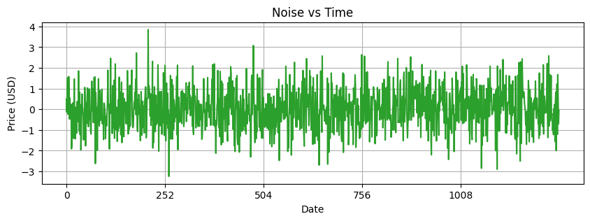
Noise

• Noise is the random fluctuations left over after trend and seasonality are removed from the original time series.

• One should not see a trend or seasonal pattern in the residuals.

• They represent short term, rather unpredictable fluctuations.

noise = np.random.normal(loc=0.0, scale=1, size=len(time))

Show code cell source

Hide code cell source

fig, ax = plt.subplots(1, 1, figsize=(10, 3))
ax.plot(time, noise, color='tab:green')
ax.set_xlabel("Date")
ax.set_ylabel("Price (USD)")
year_ticks = np.arange(0, len(time), 252)
ax.set_xticks(year_ticks)
ax.grid(True)
plt.title("Noise vs Time");

---

Decomposition Models

• Time series can be decomposed with the following models:

  • Additive decomposition

  • Multiplicative decomposition

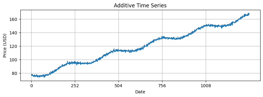
Additive model

• Additive models assume that the observed time series is the sum of its components:

\[X(t) = T(t) + S(t) + N(t)\]

• where

  • \(X(t)\) is the time series

  • \(T(t)\) is the trend

  • \(S(t)\) is the seasonality

  • \(N(t)\) is the noise

• Additive models are used when the magnitudes of the seasonal and residual values do not depend on the level of the trend.

additive = trend + seasonal + noise

Show code cell source

Hide code cell source

fig, ax = plt.subplots(1, 1, figsize=(10, 3))
ax.plot(time, additive, 'tab:blue')
ax.set_xlabel("Date")
ax.set_ylabel("Price (USD)")
year_ticks = np.arange(0, len(time), 252)
ax.set_xticks(year_ticks)
ax.grid(True)
plt.title("Additive Time Series");

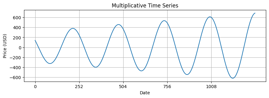
Multiplicative Model

• Assumes that the observed time series is the product of its components:

\[X(t) = T(t) \cdot S(t) \cdot R(t)\]

• It is possible to transform a multiplicative model to an additive one by applying a log transformation:

\[\log \left( T(t) \cdot S(t) \cdot R(t) \right) = \log(T(t)) + \log(S(t)) + \log(R(t))\]

• Multiplicative models are used when the magnitudes of seasonal and residual values depends on trend.

multiplicative = trend * seasonal # no noise to make the trend more pronounced

fig, ax = plt.subplots(1, 1, figsize=(10, 3))
ax.plot(time, multiplicative, 'tab:blue')
ax.set_xlabel("Date")
ax.set_ylabel("Price (USD)")
plt.title("Multiplicative Time Series")
year_ticks = np.arange(0, len(time), 252)
ax.set_xticks(year_ticks)
ax.grid(True)

For this workshop, we’ll be focusing more on the additive model.

---

Time Series Decomposition

• Now let’s go the other way.

• We have additive and multiplicative data.

• Let’s decompose them into their three components.

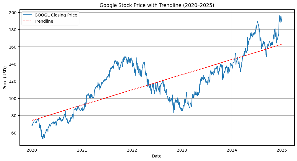
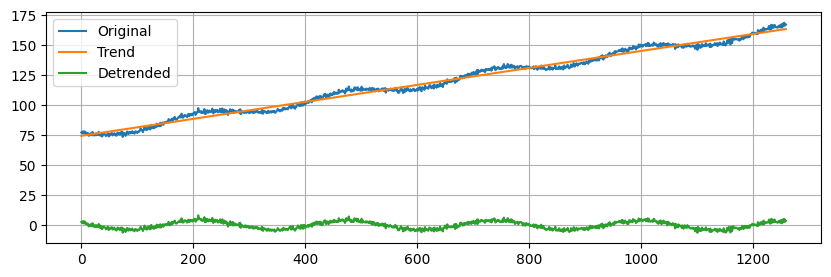
• A very simple, yet often useful, approach is to estimate a linear trend.

• A detrended time series is obtained by subtracting the linear trend from the data.

• The linear trend is computed as a 1st order polynomial.

slope, intercept = np.polyfit(np.arange(len(additive)), additive, 1) # estimate line coefficient
trend = np.arange(len(additive)) * slope + intercept                 # linear trend
detrended = additive - trend                                         # remove the trend

Show code cell source

Hide code cell source

plt.figure(figsize=(10, 3))
plt.plot(additive, label='Original')
plt.plot(trend, label='Trend')
plt.plot(detrended, label='Detrended')
plt.grid()
plt.legend();

• Next, we will use seasonal_decompose (more information here) to isolate the main time series components.

• This is a simple method that requires us to specify the type of model (additive or multiplicative) and the main period.

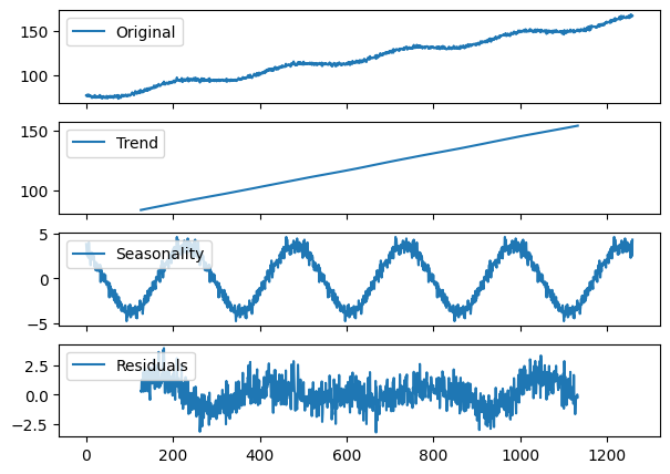
Additive Decomposition

• We need to specify an integer that represents the main seasonality of the data.

• Since the market is open for trading on 252 business days, we’ll use that as our period.

additive_decomposition = seasonal_decompose(x=additive, model='additive', period=252)

Show code cell source

Hide code cell source

# Utility function to make the plots
def seas_decomp_plots(original, decomposition):
    _, axes = plt.subplots(4, 1, sharex=True, sharey=False, figsize=(7, 5))
    axes[0].plot(original, label='Original')
    axes[0].legend(loc='upper left')
    axes[1].plot(decomposition.trend, label='Trend')
    axes[1].legend(loc='upper left')
    axes[2].plot(decomposition.seasonal, label='Seasonality')
    axes[2].legend(loc='upper left')
    axes[3].plot(decomposition.resid, label='Residuals')
    axes[3].legend(loc='upper left')
    plt.show()

seas_decomp_plots(additive, additive_decomposition)

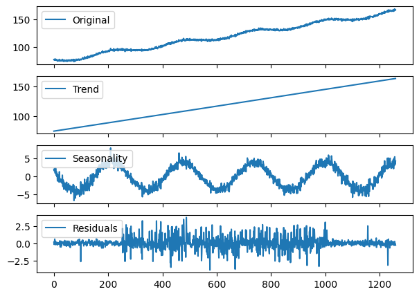
Locally estimated scatterplot smoothing (LOESS)

• Next, we try a second method called STL (Seasonal and Trend decomposition using LOESS).

stl_decomposition = STL(endog=additive, period=252, robust=True).fit()
seas_decomp_plots(additive, stl_decomposition)

Which method to use?

Use seasonal_decompose when:

• Your time series data has a clear and stable seasonal pattern and trend.

• You prefer a simpler model with fewer parameters to adjust.

• The seasonal amplitude is constant over time (suggesting an additive model).

Use STL when:

• Your time series exhibits complex seasonality that may change over time.

• You need to handle outliers effectively without them distorting the trend and seasonal components.

• You are dealing with non-linear trends and seasonality, and you need more control over the decomposition process.

---

Identifying the dominant period

• seasonal_decompose expects the dominant period as a parameter.

• In our example, the seasonal component was easy to figure out based on the behaviour of the market, but we won’t always be so lucky

• How can we find it?

• You can use one of the following techniques:

  • Plot the data and try to figure out after how many steps the cycle repeats.

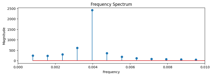
  • Use the Fast Fourier Transform on a detrended signal.

• For now, you can use the following function to compute the dominant period in the data.

Show code cell source

Hide code cell source

def fft_analysis(signal):
    
    # Linear detrending
    slope, intercept = np.polyfit(np.arange(len(signal)), signal, 1)
    trend = np.arange(len(signal)) * slope + intercept 
    detrended = signal - trend 
    
    fft_values = fft(detrended)
    frequencies = np.fft.fftfreq(len(fft_values))

    # Remove negative frequencies and sort
    positive_frequencies = frequencies[frequencies > 0]
    magnitudes = np.abs(fft_values)[frequencies > 0]

    # Identify dominant frequency
    dominant_frequency = positive_frequencies[np.argmax(magnitudes)]
    print(f"Dominant Frequency: {dominant_frequency:.3f}")

    # Convert frequency to period (e.g., days, weeks, months, etc.)
    dominant_period = 1 / dominant_frequency
    print(f"Dominant Period: {dominant_period:.2f} time units")
    
    return dominant_period, positive_frequencies, magnitudes

period, freqs, magnitudes = fft_analysis(seasonal)

Dominant Frequency: 0.004
Dominant Period: 252.00 time units

Show code cell source

Hide code cell source

# Plotting the spectrum
plt.figure(figsize=(10, 3))
plt.stem(freqs, magnitudes)
plt.title('Frequency Spectrum')
plt.xlim(0.0, 0.01) # can be moved around
plt.xlabel('Frequency')
plt.ylabel('Magnitude')
plt.show()

hourly_seasonal = 12 + np.sin(2*np.pi*time/24)

fft_analysis(hourly_seasonal);

Dominant Frequency: 0.041
Dominant Period: 24.23 time units

---

Summary

In this section we covered:

• The definition of a time series and examples of time series from the real world.

• The definition of time series analysis and examples of its application in different fields.

• A practical understanding of the three components of time series data.

• The additive and multiplicative models.

• Standard approaches to decompose a time series in its constituent parts.

---

Exercises

Exercise 1:

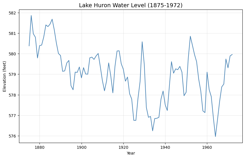
lake_huron = sm.datasets.get_rdataset("LakeHuron", "datasets").data["value"]

Perform seasonal decompositon using STL and Seasonal Decompositon, justify your choice in period (either using rational or FFT). Comment on the overall trend in the data.

Exercise 2:

passengers = sm.datasets.get_rdataset("AirPassengers", "datasets").data["value"].values

Use FFT to determine the dominant period in the data, use this to seasonally decompose the data. Once you extract the seasonality, comment on the seasonal ridership patterns.