Lecture 9 - (10/03/2026)

Today’s Topics:

K-Folds
Ridge Regression
Lasso Regression

Modeling¶

We use the train-test paradigm to help us choose a model
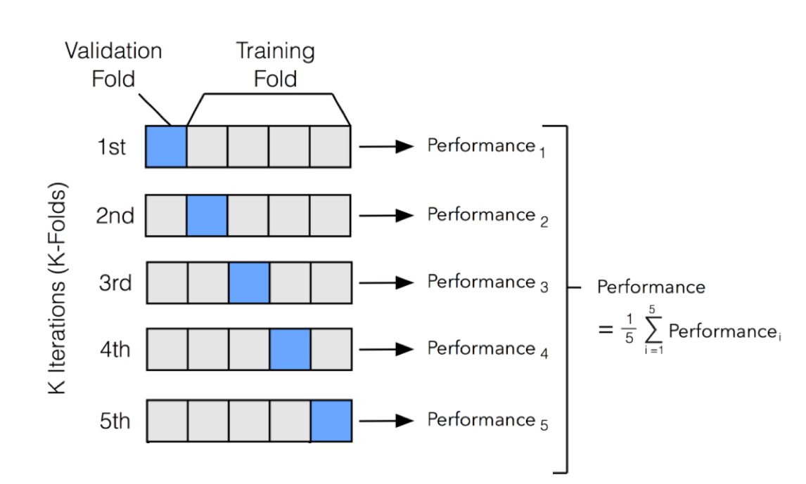
Idea: further divide the train set into separate parts where we fit the model on one part and evaluate it on another.
Above is k-fold cross-validation (where k = 5)
- Divide the train set into k roughly equal parts
- Set one fold aside to act as a test set.
- Fit all models on the remainder of the train data (the training data less the particular fold).
- Use the fold you set aside to evaluate all of these models.
- Repeat this process for a total of k times
- Combine the error in fitting each model across the folds, and choose the model with the smallest error.

import numpy as np
from sklearn.model_selection import KFold
from sklearn.linear_model import LinearRegression
from sklearn.metrics import mean_squared_error

X = np.random.rand(100, 1) * 10
y = 2 * X.squeeze() + np.random.randn(100) * 2 

kf = KFold(n_splits=5, shuffle=True, random_state=42) 

mse_scores = []

for fold, (train_index, test_index) in enumerate(kf.split(X), 1):
    X_train, X_test = X[train_index], X[test_index]
    y_train, y_test = y[train_index], y[test_index]
    
    model = LinearRegression()
    model.fit(X_train, y_train)
    
    y_pred = model.predict(X_test)
    mse = mean_squared_error(y_test, y_pred)
    mse_scores.append(mse)
    
    print(f"Fold {fold}: MSE = {mse:.3f}")

print(f"\nAverage MSE across folds: {np.mean(mse_scores):.3f}")

Fold 1: MSE = 5.299
Fold 2: MSE = 2.338
Fold 3: MSE = 4.299
Fold 4: MSE = 1.557
Fold 5: MSE = 4.148

Average MSE across folds: 3.528

Polynomial Fit¶

import numpy as np
import plotly.graph_objects as go
from sklearn.linear_model import LinearRegression
from sklearn.preprocessing import PolynomialFeatures
from sklearn.pipeline import make_pipeline

np.random.seed(0)
x = np.linspace(-5, 5, 80)
y = 0.5*x**3 - x**2 + 2*x + np.random.normal(0, 8, size=len(x))

X = x.reshape(-1,1)

lin_model = LinearRegression().fit(X, y)
y_lin = lin_model.predict(X)

poly_model = make_pipeline(PolynomialFeatures(3), LinearRegression())
poly_model.fit(X, y)
y_poly = poly_model.predict(X)

fig = go.Figure()

fig.add_trace(go.Scatter(
    x=x, y=y,
    mode='markers',
    name='Data'
))


fig.add_trace(go.Scatter(
    x=x, y=y_lin,
    mode='lines',
    name='Linear Fit'
))

fig.show()

Linear regression does not capture the relationship well.

f_{\hat\theta}(x) = \hat\theta_0 + \hat\theta_1*x

(1)

Often times we will need to use a more complex relationship, in this case a higher degree polynomial

f_{\hat\theta}(x) = \hat\theta_0 + \hat\theta_1*x + \hat\theta_2*x^2 \cdots + \hat\theta_n*x^n

(2)

import numpy as np
import plotly.graph_objects as go
from sklearn.linear_model import LinearRegression
from sklearn.preprocessing import PolynomialFeatures
from sklearn.pipeline import make_pipeline

np.random.seed(0)
x = np.linspace(-5, 5, 80)
y = 0.5*x**3 - x**2 + 2*x + np.random.normal(0, 8, size=len(x))

X = x.reshape(-1,1)

lin_model = LinearRegression().fit(X, y)
y_lin = lin_model.predict(X)

poly_model = make_pipeline(PolynomialFeatures(3), LinearRegression())
poly_model.fit(X, y)
y_poly = poly_model.predict(X)

fig = go.Figure()

fig.add_trace(go.Scatter(
    x=x, y=y,
    mode='markers',
    name='Data'
))


fig.add_trace(go.Scatter(
    x=x, y=y_lin,
    mode='lines',
    name='Linear Fit'
))

fig.add_trace(go.Scatter(
    x=x, y=y_poly,
    mode='lines',
    name='Polynomial Fit (deg=3)'
))

fig.show()

Regularization¶

Our linear model makes predictions according to the following, where $\theta$ is the model weights and $x$ is the vector of features:

f_{\hat\theta}(x) = \hat\theta * x

(3)

To fit our model, we minimize the mean squared error cost function, where X is used to represent the data matrix and y the observed outcomes:

L(\hat\theta, X, y) = \frac{1}{n} \sum_i (y_i - f_{\hat\theta}(X_i))

(4)

Regularization alters the cost function to penalize large weight values, so that the resulting model will have lower variance. THe goal is to reduce variance and still include as much information as possible.

We will cover two popular approaches: ridge & lasso regularization.

Take a look here

Ridge Regularization (L2)¶

L2 penalizes the feature engineering process by adding a penalty to the MSE cost function equivalent to the square value of the magnitude of coefficients

Linear model:

f_{\hat\theta}(x) = \hat\theta * x

(5)

MSE without regularization:

L(\hat\theta, X, y) = \frac{1}{n} \sum_i (y_i - f_{\hat\theta}(X_i))

(6)

MSE with $L_2$ regularization:

L(\hat\theta, X, y) = \frac{1}{n} \sum_i (y_i - f_{\hat\theta}(X_i)) + \lambda \sum_{j=1}{p} \hat\theta_j^2

(7)

Google colab link

import numpy as np
import plotly.graph_objects as go
from sklearn.linear_model import Ridge
from sklearn.preprocessing import PolynomialFeatures
from sklearn.pipeline import make_pipeline

np.random.seed(42)
x = np.linspace(-3, 3, 60)
y = x**3 - 2*x**2 + np.random.normal(0, 3, len(x))
X = x.reshape(-1, 1)

poly_deg = 3

alphas = np.logspace(-3, 1, 50) 
predictions = []

for alpha in alphas:
    model = make_pipeline(PolynomialFeatures(poly_deg), Ridge(alpha=alpha))
    model.fit(X, y)
    predictions.append(model.predict(X))

fig = go.Figure()

fig.add_trace(go.Scatter(x=x, y=y, mode='markers', name='Data'))

fig.add_trace(go.Scatter(x=x, y=predictions[0], mode='lines', name=f'Ridge alpha={alphas[0]:.3f}'))

steps = []
for i, alpha in enumerate(alphas):
    step = dict(
        method="update",
        args=[{"y": [y, predictions[i]]},  #
              {"title": f"Ridge Regression, alpha={alpha:.3f}"}],
        label=f"{alpha:.3f}"
    )
    steps.append(step)

sliders = [dict(
    active=0,
    currentvalue={"prefix": "Alpha: "},
    pad={"t": 50},
    steps=steps
)]

fig.update_layout(
    title=f"Ridge Regression, alpha={alphas[0]:.3f}",
    xaxis_title="x",
    yaxis_title="y",
    sliders=sliders
)

fig.show()

Stronger penalized coefficients leads to a simpler model and lower variance
Lesser penalized coefficients can fit the data very closely with low bias

Lasso Regularization (L1)¶

L1 penalizes the feature engineering process by adding a penalty to the MSE cost function equivalent to the absolute value of the magnitude of coefficients.

Linear model:

f_{\hat\theta}(x) = \hat\theta * x

(8)

MSE without regularization:

L(\hat\theta, X, y) = \frac{1}{n} \sum_i (y_i - f_{\hat\theta}(X_i))

(9)

MSE with $L_1$ regularization:

L(\hat\theta, X, y) = \frac{1}{n} \sum_i (y_i - f_{\hat\theta}(X_i)) + \lambda \sum_{j=1}{p} |\hat\theta_j|

(10)

Google colab link

import numpy as np
import plotly.graph_objects as go
from sklearn.linear_model import Lasso
from sklearn.preprocessing import PolynomialFeatures
from sklearn.pipeline import make_pipeline

np.random.seed(42)
x = np.linspace(-3, 3, 60)
y = x**3 - 2*x**2 + np.random.normal(0, 3, len(x))
X = x.reshape(-1, 1)

poly_deg = 3

alphas = np.logspace(-3, 1, 50)
predictions = []

for alpha in alphas:
    model = make_pipeline(PolynomialFeatures(poly_deg), Lasso(alpha=alpha, max_iter=10000))
    model.fit(X, y)
    predictions.append(model.predict(X))

fig = go.Figure()

fig.add_trace(go.Scatter(x=x, y=y, mode='markers', name='Data'))

fig.add_trace(go.Scatter(x=x, y=predictions[0], mode='lines', name=f'Lasso alpha={alphas[0]:.3f}'))

steps = []
for i, alpha in enumerate(alphas):
    step = dict(
        method="update",
        args=[{"y": [y, predictions[i]]},
              {"title": f"Lasso Regression, alpha={alpha:.3f}"}],
        label=f"{alpha:.3f}"
    )
    steps.append(step)

sliders = [dict(
    active=0,
    currentvalue={"prefix": "Alpha: "},
    pad={"t": 50},
    steps=steps
)]

fig.update_layout(
    title=f"Lasso Regression, alpha={alphas[0]:.3f}",
    xaxis_title="x",
    yaxis_title="y",
    sliders=sliders
)

fig.show()

Ridge Regularization (L2):

Pro: Good for grouped selection (if 2 predictors are the same, the model will have the same beta for both of them). Stable solution. Always 1 solution.
Con: The resulting model is not as simple and elegant as L1

Lasso Regularization (L2):

Pro: Sparse solution, simple model. Robust against outliers.
Con: Does not handle multi-collinearity well. If a lot of predictors are highly correlated to each other, L1 will keep only 1 of them arbitrarily. The model penalty can be too harsh and can sometimes generate multiple solutions.