Lecture 10 - (12/03/2026)

Today’s Topics:

Classification
Confusion Matrix
MNIST Example

Classification¶

In a classification problem; we predict a category, not a continuous number as we do in regression.

import pandas as pd
import numpy as np
import plotly.graph_objects as go
from sklearn.linear_model import LinearRegression

url = "https://raw.githubusercontent.com/KeithGalli/pandas/master/pokemon_data.csv"
df = pd.read_csv(url)

df["Total"] = df[["HP","Attack","Defense","Sp. Atk","Sp. Def","Speed"]].sum(axis=1)

y = df["Legendary"].astype(int)
X = df[["Total"]]

lin = LinearRegression().fit(X, y)

x_range = np.linspace(X["Total"].min(), X["Total"].max(), 300)
x_range_df = pd.DataFrame({"Total": x_range})

lin_pred = lin.predict(x_range_df)

fig = go.Figure()

fig.add_trace(go.Scatter(
    x=df["Total"],
    y=y,
    mode="markers",
    text=df["Name"],
    name="Pokemon",
    marker=dict(size=8)
))

fig.add_trace(go.Scatter(
    x=x_range.flatten(),
    y=lin_pred,
    mode="lines",
    name="Linear Regression",
    line=dict(width=4)
))

fig.update_layout(
    title="Predicting Legendary Pokemon using Regression",
    xaxis_title="Total Base Stats",
    yaxis_title="Legendary (T/F)",
)

fig.show()

The values for legendary is True/False (0/1) i.e. it is a discrete categorical variable.

When predicted values are discrete, such as legendary, then there are a lot of better options than linear regression.

Instead of a line, underlying structure is the sigmoid function

\sigma(t) = \frac{1}{1+e^{-t}}

(1)

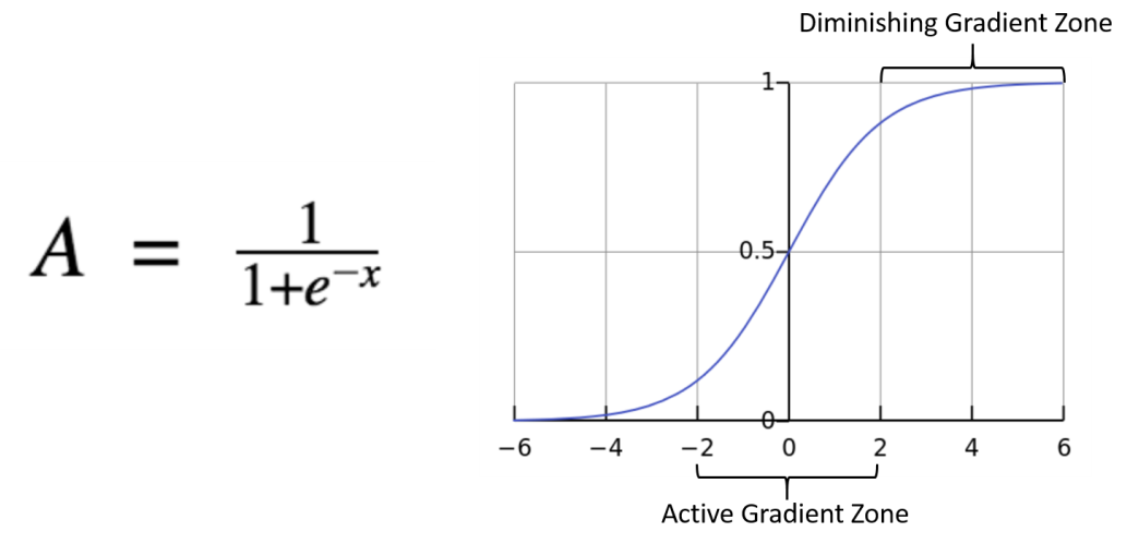
Often times we write $exp(-t) = e^{-t}
Bounded between 0 and 1
It’s derivatives make computing loss function and gradient descent straightforward

What is $\sigma(0)$ ?

\sigma(0) = \frac{1}{1+e^{-0}} = \frac{1}{1+1} = \frac{1}{2}

(2)

What is $\sigma(1)$ ?

\sigma(1) = \frac{1}{1+e^{-1}} = 0.73

(3)

What is $\sigma(1000)$ ?

\sigma(1000) = \frac{1}{1+e^{-1000}} \approx \frac{1}{1+\text{small}} = 1

(4)

What is $\sigma(-1)$ ?

\sigma(-1) = \frac{1}{1+e^{1}} = 0.27

(5)

What is $\sigma(-1000)$ ?

\sigma(-1000) = \frac{1}{1+e^{1000}} \approx \frac{1}{\text{big}} = 0

(6)

The logistic model:

f_{\hat\theta}(x) = \sigma(\hat\theta * x)

(7)

where $\hat\theta$ is a vector of values for each feature of the model.

import numpy as np
import plotly.graph_objects as go

np.random.seed(1)
x = np.random.uniform(-5,5,120)
y = (x + np.random.normal(0,2,120) > 0).astype(int)

def logistic(x, theta):
    return 1/(1+np.exp(-(theta*x)))

def cross_entropy(y, p):
    eps = 1e-9
    return -np.mean(y*np.log(p+eps) + (1-y)*np.log(1-p+eps))

x_curve = np.linspace(-5,5,300)

theta_vals = np.linspace(-4,4,60)

fig = go.Figure()

fig.add_trace(go.Scatter(
    x=x,
    y=y,
    mode="markers",
    name="data"
))

loss_values = []

for theta in theta_vals:

    p_curve = logistic(x_curve, theta)
    p_data = logistic(x, theta)

    loss = cross_entropy(y, p_data)
    loss_values.append(loss)

    fig.add_trace(go.Scatter(
        x=x_curve,
        y=p_curve,
        mode="lines",
        visible=False,
        name=f"theta={theta:.2f}"
    ))

start = len(theta_vals)//2
fig.data[start+1].visible = True

steps = []
for i,theta in enumerate(theta_vals):

    step = dict(
        method="update",
        args=[
            {"visible":[True]+[j==i for j in range(len(theta_vals))]},
            {"title":f"Logistic Regression — θ = {theta:.2f} | Cross Entropy = {loss_values[i]:.3f}"}
        ],
        label=f"{theta:.2f}"
    )

    steps.append(step)

fig.update_layout(
    sliders=[dict(
        active=start,
        currentvalue={"prefix":"θ: "},
        steps=steps
    )],
    title="Logistic Regression with Cross Entropy",
    xaxis_title="x",
    yaxis_title="Probability",
    template="plotly_white"
)

fig.show()

We will use a loss function that is suited for fitting logistic models.

The cross-entropy loss function

L(\theta, X, y) = \frac{1}{n} \sum_i (-y_i \ln(f_\theta(X_i)) - (1-y_i) \ln(1-f_\theta(X_i)))

(8)

The key intuitition is:

The more confident the model is in predicting the correct outcome, the lower the loss.
The more confident the model is in predicting the wrong outcome, the higher the loss.

The derivative is: $\sigma'(t) = \sigma(t)(1-\sigma(t))$ .

Write $\sigma_i = f_{\hat\theta}(X_i \theta)$ , then

\nabla_\theta \sigma_i = \sigma_i (1-\sigma_i) X_i

(9)

We can fit this to a model using gradient descent:

\hat\theta = \arg \min_\theta L(\theta*X, y)

(10)

import pandas as pd
import numpy as np
import plotly.graph_objects as go
from sklearn.linear_model import LinearRegression, LogisticRegression

url = "https://raw.githubusercontent.com/KeithGalli/pandas/master/pokemon_data.csv"
df = pd.read_csv(url)

df["Total"] = df[["HP","Attack","Defense","Sp. Atk","Sp. Def","Speed"]].sum(axis=1)

y = df["Legendary"].astype(int)
X = df[["Total"]].values

lin = LinearRegression().fit(X, y)
log = LogisticRegression().fit(X, y)

x_range = np.linspace(X.min(), X.max(), 300)
x_range = x_range.reshape(-1,1)

lin_pred = lin.predict(x_range)
log_pred = log.predict_proba(x_range)[:,1]

fig = go.Figure()

fig.add_trace(go.Scatter(
    x=df["Total"],
    y=y,
    mode="markers",
    text=df["Name"],
    name="Pokemon",
    marker=dict(size=8)
))

fig.add_trace(go.Scatter(
    x=x_range.flatten(),
    y=lin_pred,
    mode="lines",
    name="Linear Regression",
    line=dict(width=4)
))

fig.add_trace(go.Scatter(
    x=x_range.flatten(),
    y=log_pred,
    mode="lines",
    name="Logistic Regression",
    line=dict(width=4)
))

fig.update_layout(
    title="Legendary Pokemon: Regression vs Classification",
    xaxis_title="Total Base Stats",
    yaxis_title="Legendary (T/F)",
    template="plotly_white"
)

fig.show()

Confusion Matrix¶

import pandas as pd

data = {
    "label": ["spam","spam","spam","ham","ham","ham"],
    "email_text": [
        "Dear E-mail Owner, My name is Jeff Bezos, an American, investor, and charity donor. I'm the founder, CEO and president of Amazon.com,And Your email address has won you ( $2.500,000.00 ) Kindly get back to me , so I know your email address is valid. mrjefferybo600@gmail.com) Best Regards",
        "T-Mobile customer you may now claim your FREE CAMERA PHONE upgrade & a pay & go sim card for your loyalty. Call on 0845 021 3680.Offer ends 28thFeb",
        "U were outbid by simonwatson5120 on the Shinco DVD Plyr. 2 bid again, visit sms. ac/smsrewards 2 end bid notifications, reply END OUT",
        "I know but you need to get hotel now. I just got my invitation but i had to apologise. Cali is to sweet for me to come to some english bloke's weddin",
        "I'm really sorry i won't b able 2 do this friday.hope u can find an alternative.hope yr term's going ok:-)",
        "Lol I know! They're so dramatic. Schools already closed for tomorrow. Apparently we can't drive in the inch of snow were supposed to get"
    ]
}

df = pd.DataFrame(data)

df.style.set_properties(
    subset=["email_text"],
    **{
        "white-space": "pre-wrap",
        "max-width": "500px",
        "font-family": "monospace"
    }
).set_table_styles(
    [{"selector":"th","props":[("text-align","left")]}]
)

Our goal is to build a classifier that can identiy spam email vs non-spam (aka ham)
There are may approaches to this classic problem
We want to measure solutions on how often the model predicts correctly and incorrectly

Standard metrics measure how often our models predicts correctly and incorrectly

Many are combination of 4 basic measures:

True Positive: corectly labeled with positive class
False Negative: belongs to a positive class but mislabeled as negative
False Positive: belongs to a negative class but mislabeled as positive
True Negative: correctly labeled with negative class

Often organized in a confusion matrix: a heatmap of model predictions vs actual labels (we will go more into depth with this later)

import pandas as pd
import numpy as np
import plotly.graph_objects as go
from sklearn.linear_model import LogisticRegression

url = "https://raw.githubusercontent.com/KeithGalli/pandas/master/pokemon_data.csv"
df = pd.read_csv(url)

df["Total"] = df[["HP","Attack","Defense","Sp. Atk","Sp. Def","Speed"]].sum(axis=1)

X = df["Total"].values
y = df["Legendary"].astype(int).values

log_model = LogisticRegression()
log_model.fit(X.reshape(-1,1), y)
x_range = np.linspace(X.min(), X.max(), 300).reshape(-1,1)
log_pred = log_model.predict_proba(x_range)[:,1]

theta_vals = np.linspace(X.min(), X.max(), 50)
frames = []

for theta in theta_vals:
    preds = (X >= theta).astype(int)
    
    TN = np.sum((preds==0) & (y==0))
    FP = np.sum((preds==1) & (y==0))
    FN = np.sum((preds==0) & (y==1))
    TP = np.sum((preds==1) & (y==1))
    

    z_matrix = [[FP, TP],
                [TN, FN]] 
    
    scatter_left = [
        go.Scatter(
            x=X,
            y=y,
            mode="markers",
            text=df["Name"],
            marker=dict(
                color=["red" if p==1 else "blue" for p in preds],
                size=8
            ),
            name="Pokemon",
            xaxis="x1",
            yaxis="y1"
        ),
        go.Scatter(
            x=[theta, theta],
            y=[-0.05, 1.05],
            mode="lines",
            line=dict(color="black", width=3, dash="dash"),
            name="Theta",
            xaxis="x1",
            yaxis="y1"
        ),
        go.Scatter(
            x=x_range.flatten(),
            y=log_pred,
            mode="lines",
            line=dict(width=4, color="green"),
            name="Logistic Regression",
            xaxis="x1",
            yaxis="y1"
        )
    ]
    
    heatmap_right = [
        go.Heatmap(
            z=z_matrix,
            x=["Pred 0","Pred 1"],
            y=["Actual 1","Actual 0"],
            text=[[f"FP={FP}", f"TP={TP}"], [f"TN={TN}", f"FN={FN}"]],
            texttemplate="%{text}",
            colorscale="Blues",
            showscale=False,
            xaxis="x2",
            yaxis="y2"
        )
    ]
    
    frames.append(go.Frame(data=scatter_left + heatmap_right, name=str(theta)))

init_idx = len(theta_vals)//2
theta0 = theta_vals[init_idx]
preds0 = (X >= theta0).astype(int)

TN = np.sum((preds0==0) & (y==0))
FP = np.sum((preds0==1) & (y==0))
FN = np.sum((preds0==0) & (y==1))
TP = np.sum((preds0==1) & (y==1))
z_matrix0 = [[FP, TP],[TN, FN]]

fig = go.Figure(
    data=[
        go.Scatter(
            x=X,
            y=y,
            mode="markers",
            text=df["Name"],
            marker=dict(
                color=["red" if p==1 else "blue" for p in preds0],
                size=8
            ),
            name="Pokemon",
            xaxis="x1",
            yaxis="y1"
        ),
        go.Scatter(
            x=[theta0, theta0],
            y=[-0.05,1.05],
            mode="lines",
            line=dict(color="black", width=3, dash="dash"),
            name="Theta",
            xaxis="x1",
            yaxis="y1"
        ),
        go.Scatter(
            x=x_range.flatten(),
            y=log_pred,
            mode="lines",
            line=dict(width=4, color="green"),
            name="Logistic Regression",
            xaxis="x1",
            yaxis="y1"
        ),
        go.Heatmap(
            z=z_matrix0,
            x=["Pred 0","Pred 1"],
            y=["Actual 1","Actual 0"],
            text=[[f"FP={FP}", f"TP={TP}"], [f"TN={TN}", f"FN={FN}"]],
            texttemplate="%{text}",
            colorscale="Blues",
            showscale=False,
            xaxis="x2",
            yaxis="y2"
        )
    ],
    frames=frames
)

fig.update_layout(
    title="Pokemon Classification Using Threshold Theta",
    template="plotly_white",
    xaxis=dict(domain=[0,0.45], title="Total Stats", anchor="y1"),
    yaxis=dict(domain=[0,1], title="Legendary (0/1)", anchor="x1"),
    xaxis2=dict(domain=[0.55,1], title="Predicted", anchor="y2"),
    yaxis2=dict(domain=[0,1], title="Actual", anchor="x2"),
    sliders=[dict(
        active=init_idx,
        currentvalue={"prefix":"Theta θ: "},
        pad={"t":50},
        steps=[dict(
            method="animate",
            args=[[str(t)], {"mode":"immediate","frame":{"duration":0,"redraw":True}}],
            label=f"{t:.0f}"
        ) for t in theta_vals]
    )]
)

fig.show()

MNIST Classification¶

MNIST or Modified National Institute of Standards & Technology, is a dataset consisting of 1797 scans of handwritten digits.

Each entry has the digit represented as well as the 64 values representing the grey scale for a 8x8 image, for example:

import numpy as np
from sklearn.datasets import fetch_openml
import plotly.graph_objects as go

mnist = fetch_openml('mnist_784', version=1, as_frame=False)
X, y = mnist['data'], mnist['target'].astype(int)
X = X / 255.0

num_images = 10
images = X[:num_images].reshape(-1,28,28)
labels = y[:num_images]

init_idx = 0

fig = go.Figure(
    data=[
        go.Heatmap(
            z=images[init_idx][::-1], 
            colorscale='gray',
            showscale=False
        )
    ]
)

steps = []
for i in range(num_images):
    step = dict(
        method='update',
        args=[{'z':[images[i][::-1]]}, 
              {'title': f"MNIST Image Index {i} (Label: {labels[i]})"}],
        label=str(i)
    )
    steps.append(step)

sliders = [dict(
    active=0,
    currentvalue={"prefix":"Image Index: "},
    pad={"t":50},
    steps=steps
)]

fig.update_layout(
    sliders=sliders,
    title=f"MNIST Image Index {init_idx} (Label: {labels[init_idx]})",
    xaxis=dict(showticklabels=False),
    yaxis=dict(showticklabels=False)
)

fig.show()

General Strategy:

Clean the data
Split the data into training and testing subsets
Instantiate and fit the model to the training data (validate/tune model parameters)
Test the model

from sklearn.datasets import fetch_openml
from sklearn.linear_model import LogisticRegression
from sklearn.model_selection import train_test_split
from sklearn.metrics import accuracy_score, confusion_matrix, classification_report

mnist = fetch_openml('mnist_784', version=1, as_frame=False)
X, y = mnist['data'], mnist['target'].astype(int)
X = X / 255.0

X_train, X_test, y_train, y_test = train_test_split(X, y, test_size=0.2, random_state=42)

log_clf = LogisticRegression(max_iter=100)
log_clf.fit(X_train, y_train)

y_pred = log_clf.predict(X_test)
print("Accuracy:", accuracy_score(y_test, y_pred))

Accuracy: 0.9202857142857143

/Users/ko/Documents/data-science-sp26/.venv/lib/python3.13/site-packages/sklearn/linear_model/_logistic.py:406: ConvergenceWarning:

lbfgs failed to converge after 100 iteration(s) (status=1):
STOP: TOTAL NO. OF ITERATIONS REACHED LIMIT

Increase the number of iterations to improve the convergence (max_iter=100).
You might also want to scale the data as shown in:
    https://scikit-learn.org/stable/modules/preprocessing.html
Please also refer to the documentation for alternative solver options:
    https://scikit-learn.org/stable/modules/linear_model.html#logistic-regression

import numpy as np
from sklearn.datasets import fetch_openml
from sklearn.linear_model import LogisticRegression
from sklearn.model_selection import train_test_split
import plotly.graph_objects as go
from plotly.subplots import make_subplots

mnist = fetch_openml('mnist_784', version=1, as_frame=False)
X, y = mnist['data'], mnist['target'].astype(int)
X = X / 255.0

X_train, X_test, y_train, y_test = train_test_split(X, y, test_size=0.2, random_state=42)

log_clf = LogisticRegression(max_iter=100)
log_clf.fit(X_train, y_train)

init_idx = 0
digit_image = X_test[init_idx].reshape(28,28)
probs = log_clf.predict_proba(X_test[init_idx].reshape(1,-1))[0]

fig = make_subplots(
    rows=1, cols=2,
    column_widths=[0.4,0.6],
    specs=[[{"type":"heatmap"}, {"type":"bar"}]],
    subplot_titles=["MNIST Digit", "Predicted Probabilities"]
)

fig.add_trace(
    go.Heatmap(
        z=digit_image[::-1],
        colorscale="gray",
        showscale=False
    ),
    row=1, col=1
)

fig.add_trace(
    go.Bar(
        x=list(range(10)),
        y=probs,
        text=[f"{p:.2f}" for p in probs],
        textposition="auto",
        name="Probabilities"
    ),
    row=1, col=2
)

steps = []
for i in range(100):
    digit_i = X_test[i].reshape(28,28)
    probs_i = log_clf.predict_proba(X_test[i].reshape(1,-1))[0]
    step = dict(
        method="update",
        args=[
            {"z":[digit_i[::-1], None], "y":[None, probs_i], "text":[None, [f"{p:.2f}" for p in probs_i]]}
        ],
        label=str(i)
    )
    steps.append(step)

sliders = [dict(active=init_idx, currentvalue={"prefix":"Test index: "}, pad={"t":50}, steps=steps)]

fig.update_layout(
    sliders=sliders,
    title="MNIST Logistic Regression Prediction Demo",
    xaxis=dict(showticklabels=False),
    yaxis=dict(showticklabels=False)
)

fig.show()

/Users/ko/Documents/data-science-sp26/.venv/lib/python3.13/site-packages/sklearn/linear_model/_logistic.py:406: ConvergenceWarning:

lbfgs failed to converge after 100 iteration(s) (status=1):
STOP: TOTAL NO. OF ITERATIONS REACHED LIMIT

Increase the number of iterations to improve the convergence (max_iter=100).
You might also want to scale the data as shown in:
    https://scikit-learn.org/stable/modules/preprocessing.html
Please also refer to the documentation for alternative solver options:
    https://scikit-learn.org/stable/modules/linear_model.html#logistic-regression