Lecture 7 - (03/03/2026)

Today’s Topics:

Multiple Linear Regression
Gradient Descent
Feature Engineering

Multiple Linear Regression¶

Linear Algebra¶

So far we have worked with 1-D linear regression where each observation has only one feature which allows us to use simple pointwise multiplication for each operation.

y_i = \beta_0 + \beta_1 x_{i_1} + \beta_2 x_{i_2} + \cdots + \beta_n x_{i_n} + \varepsilon_i

(1)

which can also be represented as

y_i=\begin{bmatrix} 1 & x_{i_1} & x_{i_2} & \cdots & x_{i_n} \end{bmatrix} \begin{bmatrix} \beta_0 \\ \beta_1 \\ \beta_2 \\ \vdots \\ \beta_n \end{bmatrix} + \varepsilon_i

(2)

Since we are working with dataframes that have multiple features, we will need to introduce something a little bit more powerful for our linear regression, matrices:

\begin{bmatrix} y_1 \\ y_2 \\ \vdots \\ y_m \end{bmatrix} = \begin{bmatrix} 1 & x_{11} & x_{12} & \cdots & x_{1n} \\ 1 & x_{21} & x_{22} & \cdots & x_{2n} \\ \vdots & \vdots & \vdots & \ddots & \vdots \\ 1 & x_{m1} & x_{m2} & \cdots & x_{mn} \end{bmatrix} \begin{bmatrix} \beta_0 \\ \beta_1 \\ \beta_2 \\ \vdots \\ \beta_n \end{bmatrix} + \begin{bmatrix} \varepsilon_1 \\ \varepsilon_2 \\ \vdots \\ \varepsilon_m \end{bmatrix}

(3)

Despite the change in notation, they behave the same way, and we can simplify this by writing:

\hat y = wx + b

(4)

Feature Selection¶

In many data sets there may be several predictor variables that have an effect on a response variable. In fact, the interaction between variables may also be used to predict response. When we incorporate these additional predictor variables into the analysis, the model is called multiple linear regression.

import numpy as np
import pandas as pd
from sklearn import datasets
from sklearn.model_selection import train_test_split
from sklearn import linear_model

cali = datasets.fetch_california_housing()
X = pd.DataFrame(cali.data, columns=cali.feature_names)
y = pd.Series(cali.target)

X.head()

Loading...

y.head()

0    4.526
1    3.585
2    3.521
3    3.413
4    3.422
dtype: float64

X.describe()

Loading...

For each row of X and y it can be interpreted as:

Entry 0 of X:

Median Income: $83,252
Age of Household: 41 years
Average Rooms: 6.98
Aveage Bedrooms: 1.02
Population: 322
Average Occupiants: 2.55 persons
Latitude: 37.88
Longitude: -122.23

Entry 0 of y:

House Price: $452,600

What features in X do you think contribute to the value of y?

Let’s guess that age of the house, number of rooms, and number of bedrooms all contribute to it.

Our new linear regression function will be:

PRICE = \beta_0 + \beta_1 * \text{AGE} + \beta_2 * \text{ROOMS} + \beta_3 * \text{BEDRM}

(5)

One of the most important things to notice about this equation is that each variable makes a contribution independently of the other variables. This is called additivity: the effects of predictor variable are added together to get the total effect on PRICE.

linreg = linear_model.LinearRegression()

linreg.fit(X[['MedInc', 'HouseAge', 'AveRooms', 'AveOccup']], y)

Loading...

linreg.score(X[['MedInc', 'HouseAge', 'AveRooms', 'AveOccup']], y)

0.5137125846287833

Interaction Events¶

Suppose we discovered that people who live in upper california (higher latitude) and had older houses (higher house age) tended to have cheaper houses, but people who lived in lower california with newer houses had more expensive houses. This chould indicate an interaction event on the response. When there is an interaction effect, the effects of the variables involved are not additive.

Different numbers of variables can be involved in an interaction. When two features are involved in the interaction it is called a two-way interaction. There are three-way and higher interactions possible as well, but they are less common in practice. The full model includes main effects and all interactions.

Often in practice we fit the full model to check for significant interaction effects. If there are no interactions that are significantly different from zero, we can drop the interaction terms and fit the main effects model to see which of those effects are significant.

PRICE = \beta_0 + \beta_1 * \text{AGE} * \text{LAT} + \beta_2 * \text{ROOMS} + \beta_3 * \text{BEDRM}

(6)

Collinearity¶

Collinearity(or Multicollinearity) occurs when two variables or features are linearly related, i.e. they have very strong correlation between them (close to -1 or 1). Practically this means that some of the independent variables are measuring the same thing and are not needed. In terms of linear algebra, this is considered a linear dependance, and one of the variables can be removed.

In our case, rooms and bedrooms are likely linearly related therefore it would be redundant to include both of them in our model so we can opt to remove one of them.

PRICE = \beta_0 + \beta_1 * \text{AGE} * \text{LAT} + \beta_2 * \text{ROOMS}

(7)

Gradient Descent¶

When we are modeling a graph we tend to follow the following procedure:

Split your data into pieces for training & validation
Select a model
Select a loss function
Minimize the loss function, using training data.
Validate your model with reserved test data

But how do we minimize the loss function?

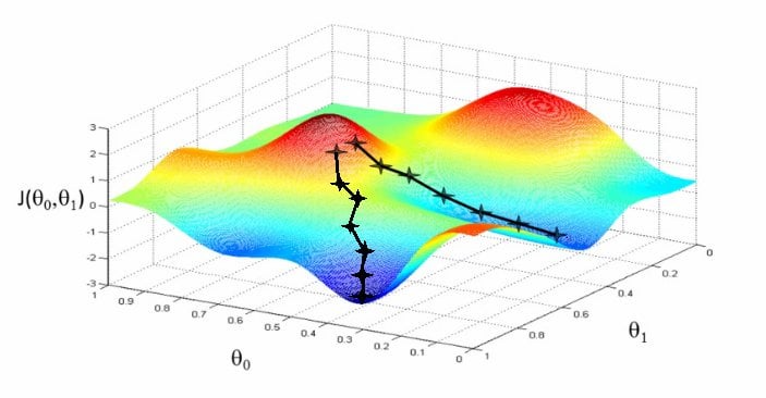
The idea:

Slide down the hill in the direction of least resistance.

Moving forward, to find the lowest error(deepest point) in the loss function(with respect to one weight), we need to tweak the parameters of the model. Using calculus, we know that the slope of a function is the derivative of the function with respect to a value. This slope always points to the nearest valley!

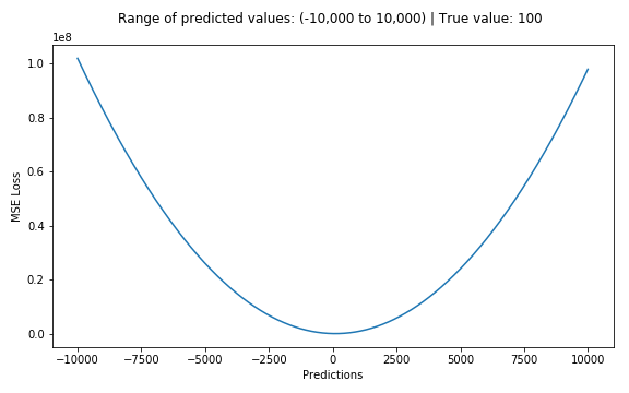
If we try to think of it in visual terms, our training data set is scattered on the x-y plane. We are trying to make a straight line (defined by $\hat y$ ) which passes through these scattered data points.

Our objective is to get the best possible line. The best possible line will be such so that the average squared vertical distances of the scattered points from the line will be the least. Ideally, the line should pass through all the points of our training data set. In such a case, the value of the error function will be 0.

MSE = \frac{1}{n} (y_i - \hat y)^2

(8)

= \frac{1}{n} (y_i - (wx_i + b))^2

(9)

def mse_loss(x, y, w, b):
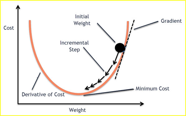
    return np.mean(np.square(y - (w * x + b)))

In each epoch of gradient descent, a parameter is updated by subtracting the product of the gradient of the function and the learning rate $lr$ . The learning rate controls how much the parameters should change. Small learning rates are precise, but are slow. Large learning rates are fast, but may prevent the model from finding the local extrema.

$$ X_{n+1} = X_n - lr* \frac{\partial}{\partial X} f(X_n)

Since we are finding the optimal slope ( $w$ ) and y-intercept ( $b$ ) for our linear regression model, we must find the partial derivatives of the loss function with respect to $w$ and $b$ .

We repeate this process until there is no difference between $X_{n+1}$ and $X_n$ which implies that the model has converged to some minimum loss value.

Enough about this, let’s practice it with a game