Lecture 5 - (19/02/2026)

Today’s Topics:

Linear Modeling
Scikit Learn
Project Overview

Recap¶

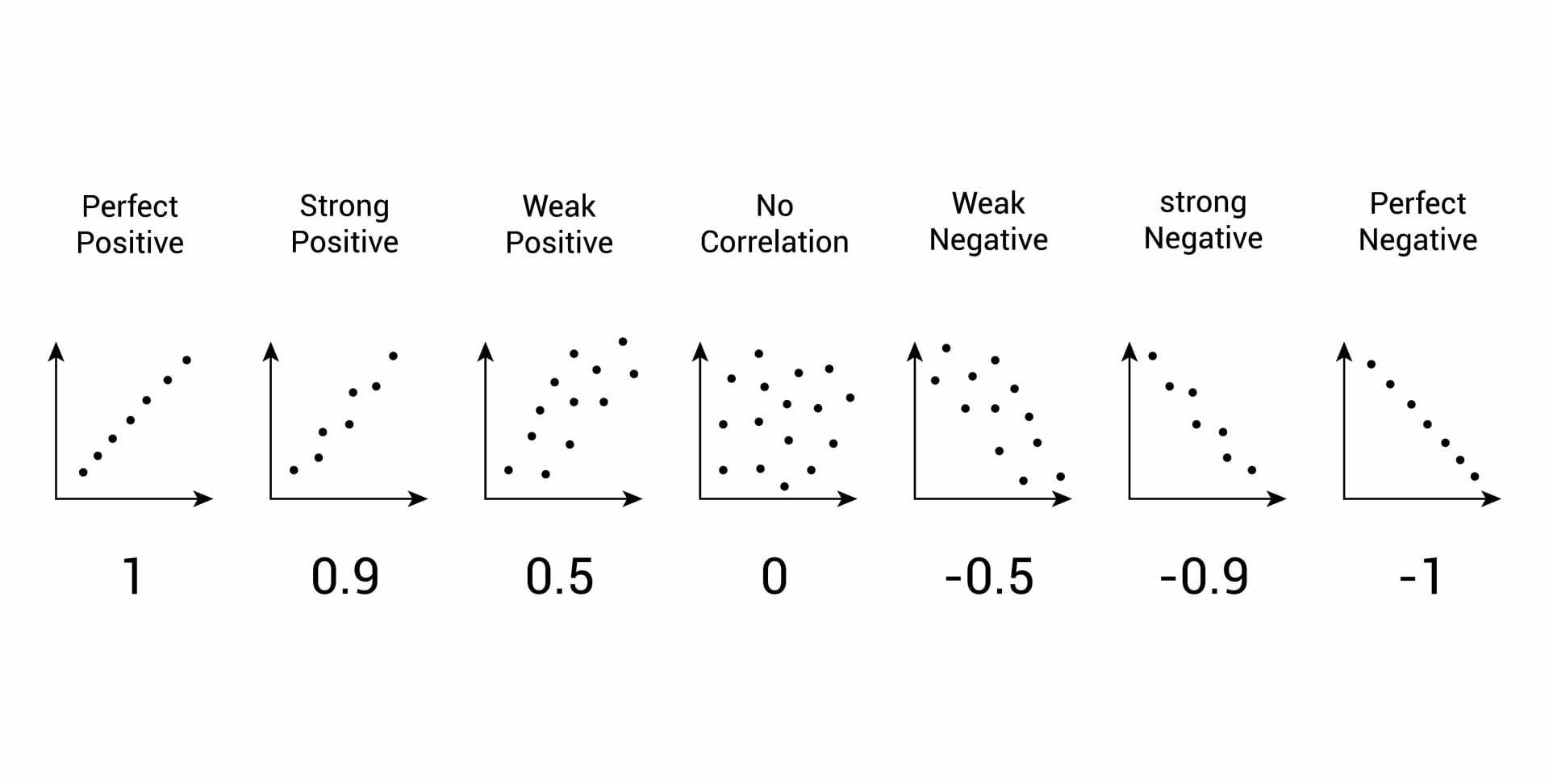
Last time we explored the correlation coefficient which gives a single number measuring the association between the variables.

explored a method to make simple predictions called linear regression in the form of $y=mx+b$

https://www.researchgate.net/publication/381857634/figure/fig1/AS:11431281257626828@1719839742106/Linear-regression-model.png

and we can use the differences (green line) or residuals can give us additional information

Linear Modeling¶

We can score each line with how close the actual and predicted y-values are, using RMSE for the loss function.

The line with the best score is determined as the regression line.

We can visualize this process here

Our goal in linear regression is to seek the line $y=mx+b$ that minimizes the least square errors

That is to say, the line that minimizes the mean of the MSE(mean squared errors) for all lines.

When x and y are in standard units, regression line is:

y = r*x + 0

(1)

Let’s try a game (make sure to record your scores)!

Modeling should generally consist of three main steps

Select a model (in our case linear regression)
Select a loss function (in our case RMSE)
Minimize the loss function

We also need to prep our data for prediction, adding in those steps:

Split your data into pieces for training & validation.
Select a model (in our case linear regression)
Select a loss function (in our case RMSE)
Minimize the loss function, using the training data
Validate your model with the reserved test data

Scikit Learn¶

Scikit learn is:

Toolkit for predictive data analysis.
Built on NumPy, SciPy, and matplotlib
Open source, commercially usable (BSD license)
Easy ‘building blocks’ for analysis, many tutorials & recipes

!pip install scikit-learn  # to install

def matprint(mat, fmt="g"):
    col_maxes = [max([len(("{:"+fmt+"}").format(x)) for x in col]) for col in mat.T]
    for x in mat:
        for i, y in enumerate(x):
            print(("{:"+str(col_maxes[i])+fmt+"}").format(y), end="  ")
        print("")

import numpy as np
import matplotlib.pyplot as plt
from sklearn import linear_model, datasets
from sklearn.model_selection import train_test_split
X,y = datasets.load_diabetes(return_X_y=True)

matprint(X[:20])

  0.0380759   0.0506801    0.0616962    0.0218724   -0.0442235    -0.0348208   -0.0434008  -0.00259226   0.0199075   -0.0176461  
-0.00188202  -0.0446416   -0.0514741   -0.0263275  -0.00844872    -0.0191633    0.0744116   -0.0394934  -0.0683315    -0.092204  
  0.0852989   0.0506801    0.0444512  -0.00567042   -0.0455995    -0.0341945   -0.0323559  -0.00259226  0.00286131   -0.0259303  
 -0.0890629  -0.0446416    -0.011595   -0.0366561    0.0121906     0.0249906   -0.0360376    0.0343089   0.0226877  -0.00936191  
 0.00538306  -0.0446416   -0.0363847    0.0218724   0.00393485     0.0155961   0.00814208  -0.00259226  -0.0319876   -0.0466409  
 -0.0926955  -0.0446416   -0.0406959   -0.0194418   -0.0689906    -0.0792878    0.0412768   -0.0763945  -0.0411762   -0.0963462  
 -0.0454725   0.0506801   -0.0471628    -0.015999   -0.0400956       -0.0248  0.000778808   -0.0394934  -0.0629169   -0.0383567  
  0.0635037   0.0506801  -0.00189471    0.0666294    0.0906199      0.108914    0.0228686    0.0177034  -0.0358162   0.00306441  
  0.0417084   0.0506801    0.0616962   -0.0400989   -0.0139525    0.00620169   -0.0286743  -0.00259226  -0.0149597    0.0113486  
 -0.0709002  -0.0446416    0.0390622   -0.0332132   -0.0125766    -0.0345076   -0.0249927  -0.00259226   0.0677371    -0.013504  
  -0.096328  -0.0446416   -0.0838084   0.00810098    -0.103389    -0.0905612   -0.0139477   -0.0763945  -0.0629169   -0.0342146  
  0.0271783   0.0506801    0.0175059   -0.0332132  -0.00707277     0.0459715   -0.0654907      0.07121  -0.0964349   -0.0590672  
  0.0162807  -0.0446416     -0.02884  -0.00911327  -0.00432087   -0.00976889    0.0449585   -0.0394934  -0.0307479   -0.0424988  
 0.00538306   0.0506801  -0.00189471   0.00810098  -0.00432087    -0.0157187  -0.00290283  -0.00259226   0.0383939    -0.013504  
   0.045341  -0.0446416   -0.0256066   -0.0125561    0.0176944  -6.12836e-05    0.0817748   -0.0394934  -0.0319876   -0.0756356  
 -0.0527376   0.0506801   -0.0180619    0.0804009    0.0892439      0.107662   -0.0397192     0.108111   0.0360603   -0.0424988  
-0.00551455  -0.0446416    0.0422956    0.0494152    0.0245741    -0.0238606    0.0744116   -0.0394934    0.052277    0.0279171  
  0.0707688   0.0506801    0.0121169    0.0563009    0.0342058     0.0494162   -0.0397192    0.0343089    0.027364   -0.0010777  
 -0.0382074  -0.0446416   -0.0105172   -0.0366561   -0.0373437    -0.0194765   -0.0286743  -0.00259226  -0.0181137   -0.0176461  
 -0.0273098  -0.0446416   -0.0180619   -0.0400989  -0.00294491    -0.0113346    0.0375952   -0.0394934  -0.0089434   -0.0549251

y[:20]

array([151.,  75., 141., 206., 135.,  97., 138.,  63., 110., 310., 101.,
        69., 179., 185., 118., 171., 166., 144.,  97., 168.])

X.shape, y.shape

((442, 10), (442,))

# split the data into a training and validation set

X_train, X_test, y_train, y_test = train_test_split(X,y,test_size=0.33,random_state=42)

X_train.shape, y_train.shape

((296, 10), (296,))

X_test.shape, y_test.shape

((146, 10), (146,))

# select a model

reg = linear_model.LinearRegression()

# select a loss functon (defaults to RMSE)

# minimize the loss function using the training data
reg.fit(X_train, y_train)

# validate the model with the reserved test data
y_pred = reg.predict(X_test)

from sklearn.metrics import mean_squared_error, r2_score

print(f"Mean squared error: {mean_squared_error(y_test, y_pred):.2f}")
print(f"Coefficient of determination: {r2_score(y_test, y_pred):.2f}")

Mean squared error: 2817.81
Coefficient of determination: 0.51

# visualisation

X, y = datasets.load_diabetes(return_X_y=True)
X = X[:, [2]]  # Use only one feature
X_train, X_test, y_train, y_test = train_test_split(X, y, test_size=20, shuffle=False)
regressor = linear_model.LinearRegression().fit(X_train, y_train)

fig, ax = plt.subplots(ncols=2, figsize=(10, 5), sharex=True, sharey=True)

ax[0].scatter(X_train, y_train, label="Train data points")
ax[0].plot(
    X_train,
    regressor.predict(X_train),
    linewidth=3,
    color="tab:orange",
    label="Model predictions",
)
ax[0].set(xlabel="Feature", ylabel="Target", title="Train set")
ax[0].legend()

ax[1].scatter(X_test, y_test, label="Test data points")
ax[1].plot(X_test, regressor.predict(X_test), linewidth=3, color="tab:orange", label="Model predictions")
ax[1].set(xlabel="Feature", ylabel="Target", title="Test set")
ax[1].legend()

fig.suptitle("Linear Regression")

plt.show()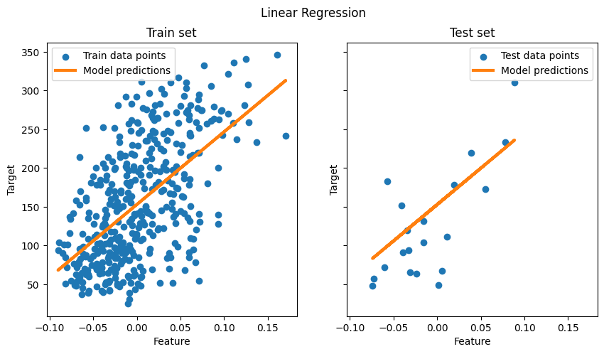

Loss function Properties:

Seeking the minimum of the loss function over the inputs
Nice way to find minimums of functions is via calculus.
- Take the derivatives and look at the 0’s
With the absolute values, MAE is not differentiable.
- Limits are different from left and right
MAE is minimal at the median of y, $\theta = median(y)$ .
MSE is the sum of quadratics, so, differentiable, and is minimal at the mean of y, $\theta=mean(y)$

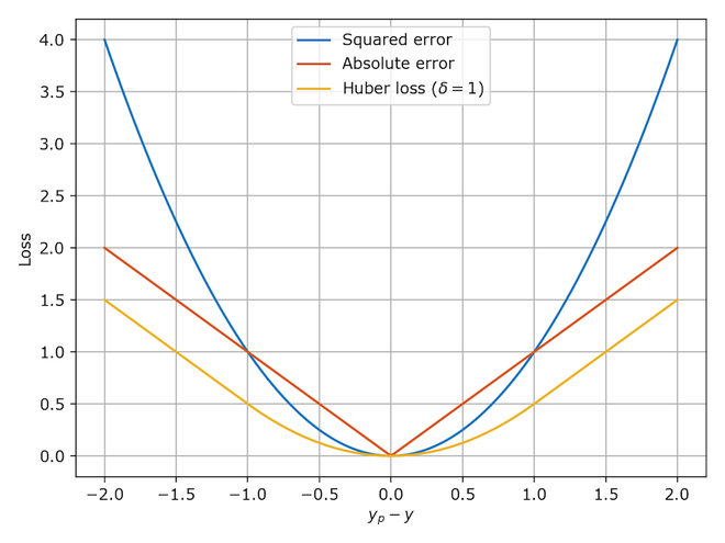
Huber combined good properties of both.

Mean Squared Error

\mathrm{MSE} = \frac{1}{n}\sum_{i=1}^{n} (y_i - \theta)^2

(2)

Root Mean Squared Error

\mathrm{RMSE} = \sqrt{\frac{1}{n}\sum_{i=1}^{n} (y_i - \theta)^2}

(3)

Mean Absolute Error

\mathrm{MAE} = \frac{1}{n}\sum_{i=1}^{n} \lvert y_i - \theta \rvert

(4)

Project Overview¶

Deadline	Deliverable	Points	Submission Window Opens
Tuesday, 3 March	Opt-in	0	Tuesday, 24 Febuary
Thursday, 19 March	Proposal	50	Tuesday, 10 March
Tuesday, April 7	Interim Check-In	25	Tuesday, March 31
TBA	Complete Project	100	TBA
TBA	Presentation Slides	25	TBA
	Total Points	200

The optional project must:

Use publicly available data, ideally from Kaggle or NYC Open Data.
Employ a predictive model.
Visualizations that include summary statistics plots, map graphs, and model perfomance plots.