Lecture 3 - (05/02/2026)

Today’s Topics:¶

Lambda functions
Data Representation and Pandas
Loss Functions

Lambda functions¶

Lambda expressions are “small anonymous functions”
Mainly used for small and temporary tasks.
Very common for apply() (and map() & reduce()).
They can be stored as a variable and used as a function

f = lambda x : x**2
f(4), f(6), f(8), f(10)

(16, 36, 64, 100)

pairs = [('Alice', 94), ('Bob', 87), ('Charlie', 78), ('David', 88), ('Emily', 83)]
pairs.sort(key = lambda pair : pair[1])
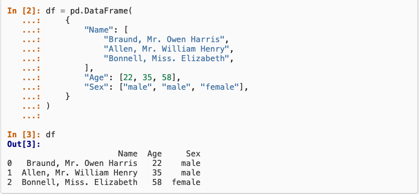
pairs

[('Charlie', 78), ('Emily', 83), ('Bob', 87), ('David', 88), ('Alice', 94)]

Example: create a new column that is true a pokemon has two types

import pandas as pd
df = pd.read_csv("https://gist.githubusercontent.com/armgilles/194bcff35001e7eb53a2a8b441e8b2c6/raw/92200bc0a673d5ce2110aaad4544ed6c4010f687/pokemon.csv")
df.head()

Loading...

df = df.assign(two_type_boolean = lambda row : (row["Type 2"].notna()))
df.head()

Loading...

Pandas¶

We will use the popular Python Data Analysis Library (Pandas).
Open source and freely available, in collab & most distributions.
Pandas documentation: Getting Started

Reading and Writing to CSV’s

import pandas as pd
df = pd.read_csv('infile.csv')
pass
pass
pass
df.to_csv('outfile.csv', index=False)

Constructing from a dictionary:

Selecting by label¶

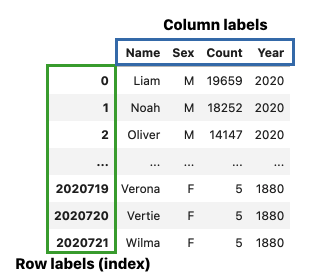
baby = pd.read_csv("https://raw.githubusercontent.com/jsvine/babynames/refs/heads/master/data/name-counts.csv")
baby.head()

Loading...

#  The first arguement is the row label
#       \/ 
baby.loc[1, 'name']
#            /\
#       The second arguement is the column label

'Anna'

Selects the entry in row 1, column “name” which is ‘Anna’

We can also select a range of values

baby.loc[1:3, 'name':'count'] # is inclusive!

Loading...

# Just extract the name and count columns
baby.loc[:, ['name', 'count']]
#            list of column labels

Loading...

What happens if you use single versus double brackets?

# Shorthand for baby.loc[:, 'name']
type(baby['name']), baby['name']

(pandas.Series,
 0               Mary
 1               Anna
 2               Emma
 3          Elizabeth
 4             Minnie
              ...    
 1758725        Zylin
 1758726       Zymari
 1758727        Zyrin
 1758728        Zyrus
 1758729    Zytaevius
 Name: name, Length: 1758730, dtype: str)

Returns a series (pandas equivalent to a list/vector) and not a entire dataframe

Boolean Selection¶

We can build more complex selections using Boolean selection
Create a Series of Booleans that selects rows where the Series is True:

baby.loc[baby['year'] == 2000, :]
# baby.loc[baby['year'] == 2000] also works here

Loading...

baby.loc[baby['count'] == 5]

Loading...

Modeling and Estimation¶

Essentially, all models are wrong, but some are useful. - George Box, Statistician (1919-2013)

A model is an idealized representation of a system.
Example: weather forecasts make predictions that are often (in)correct but sometimes not.

url = "https://raw.githubusercontent.com/mwaskom/seaborn-data/master/tips.csv"
tips = pd.read_csv(url)

Code for histogram:

# for class
import seaborn as sns
sns.histplot(tips['tip'], bins=25)

<Axes: xlabel='tip', ylabel='Count'>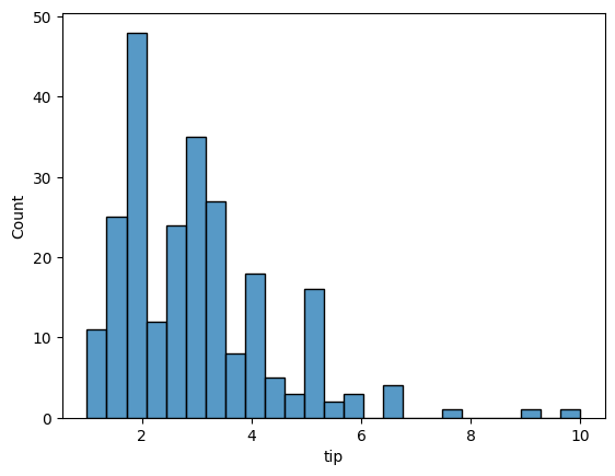

# more advanced visualization
# variable binning

import plotly.express as px

fig = px.histogram(tips, x="tip")
fig.update_layout(
    sliders=[{
        "active": 25,
        "currentvalue": {"prefix": "Number of bins: "},
        "pad": {"t": 50},
        "steps": [
            {
                "label": str(b),
                "method": "restyle",
                "args": [{"nbinsx": b}]
            }
            for b in range(5, 51)
        ]
    }]
)
fig.show()

Loading...

px.scatter(tips, x='total_bill', y='tip')

Loading...

import plotly.figure_factory as ff

tips['percent'] = tips['tip'] / tips['total_bill'] * 100
fig = ff.create_distplot([tips['percent']], ["Percent Tips"])
fig.show()

Loading...

What would be a good estimate, $\theta$ , for percent tip?

Plotly related reading:

Loss Functions¶

To quantify how good an estimate is, we will use loss functions.
A loss function:
- takes in an estimate $\theta$ and the points in our dataset, $y_1, y_2, ..., y_n$ , and
- outputs a single number, the loss, that measures how well $\theta$ fits the data
The choice of loss function affects the downstream analysis.

Let’s try something simple: taking the minimum difference, that is

f(\theta, y_1, y_2, \cdots, y_n) = \min(y_1 - \theta, y_2 - \theta, \cdots, y_n - \theta)

(1)

Suppose $\theta = 15$ , then:

tips['percent'] = tips['tip'] / tips['total_bill'] * 100
fig = ff.create_distplot([tips['percent']], ["Percent Tips"])
fig.add_vline(x=15, line_color = 'purple', line_dash = 'dash')
fig.show()

Loading...

For tips, this would be for $\theta = 15$ :

= \min(−9.055327, 1.054159, 1.658734, \cdots , 0.974441)

(2)

= −11.436186414864453

(3)

Doesn’t capture much information about the values... just the smallest one

Let’s sum up the differences instead:

f(\theta, y_1, y_2, \cdots, y_n) = (y_1 - \theta) + (y_2 - \theta) + \cdots + (y_n - \theta)

(4)

For tips, this would be $\theta = 15$ :

= −9.055327 + 1.054159 + 1.658734 + \cdots + 0.974441

(5)

= 263.58299402911507

(6)

With the negative values, the differences are cancelling out.

To avoid the differences cancelling, make the differences positive:

Use absolute value of the differences:
$f(\theta, y_1, y_2, \cdots, y_n) = |y_1 - \theta| + |y_2 - \theta| + \cdots + |y_n - \theta|$
(7)
Square the differences:
$f(\theta, y_1, y_2, \cdots, y_n) = (y_1 - \theta)^2 + (y_2 - \theta)^2 + \cdots + (y_n - \theta)^2$
(8)

Now we’re getting somewhere! We should normalize the number so we can compare it between different sample sizes.

Mean Absolute Error: Use average of absolute value of the differences:

f(\theta, y_1, y_2, \cdots, y_n) = \frac{1}{n}(|y_1 - \theta| + |y_2 - \theta| + \cdots + |y_n - \theta|)

(9)

Mean Squared Error: Use average of the square the differences:

f(\theta, y_1, y_2, \cdots, y_n) = \frac{1}{n}((y_1 - \theta)^2 + (y_2 - \theta)^2 + \cdots + (y_n - \theta)^2)

(10)

Later we will learn loss functions for more complex models

Applying functions to Series¶

Pandas has a mechanism for applying a function to every element in a Series, called apply
Similar to aggregate functions, but slower and works on a single column of data.

names = baby['name']
names.apply(len)

0          4
1          4
2          4
3          9
4          6
          ..
1758725    5
1758726    6
1758727    5
1758728    5
1758729    9
Name: name, Length: 1758730, dtype: int64

We can use built in functions... or we can write our own:

first_letter = lambda x : x[0]

names.apply(first_letter)

0          M
1          A
2          E
3          E
4          M
          ..
1758725    Z
1758726    Z
1758727    Z
1758728    Z
1758729    Z
Name: name, Length: 1758730, dtype: str

Since apply returns a series, we can use it to create a new column in our dataframe.

baby['firsts'] = names.apply(first_letter)
baby.head()

Loading...

alternatively:

baby = baby.assign(firsts=names.apply(first_letter))
baby.head()

Loading...

Last thing, let’s step by step take the MSE for our tips dataframe

This will be our pipeline:

Calculate the difference between each item and 15
Calculate the squared value of each of the values in difference
Sum the squared row
Divide by the number of rows we have

n = 15
difference_fn = lambda x : x-15

tips = tips.assign(difference=tips['percent'].apply(difference_fn))
tips.head()

Loading...

squared_fn = lambda x : x**2

tips = tips.assign(squared=tips['difference'].apply(squared_fn))
tips.head()

Loading...

tips['squared'].sum() / tips['squared'].count()

np.float64(38.31223773226083)

Let’s combine this into one function:

def calculate_loss(df, theta, func = lambda x : x**2):
    difference_fn = lambda x : x-theta
    
    df = df.assign(difference=df['percent'].apply(difference_fn))
    df = df.assign(new=df['difference'].apply(func))
    return df['new'].sum() / df['new'].count()

calculate_loss(tips, 10)

np.float64(74.11481945476554)

import numpy as np

thetas = np.linspace(0, 32, 100)
losses = [calculate_loss(tips, theta) for theta in thetas]

px.line(x=thetas,y=losses)

Loading...

min_idx = np.argmin(losses)
print(f'Minimum Theta: {thetas[min_idx]}')
print(f'Minimum MSE: {losses[min_idx]}')

Minimum Theta: 16.161616161616163
Minimum MSE: 37.15189913598053