Lecture 21 - (12/05/26)
Today’s Topics:
Deep Neural Network Recap
Recurrent Neural Networks
Long Short Term Memory
DNN Recap
A simple neural network consists of three different parts namely Parameters, Linear, and None-Linear (Activation Function) parts:
First, a weight is being applied to each input to an artificial neuron.
Second, the inputs are multiplied by their weights, and then a bias is applied to the outcome. This is called the weighted sum.
Third, the weighted sum is processed via an activation function, as a non-linear function.
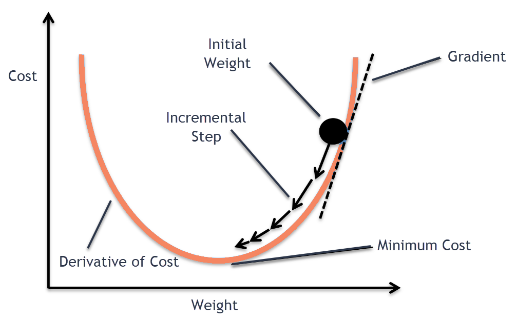
The neural network can compare the outputs of its nodes with the desired values using a property known as the delta rule, allowing the network to alter its weights through training to create more accurate output values. This training and learning procedure results in gradient descent.
The technique of updating weights in multi-layered perceptrons is virtually the same, however, the process is referred to as back-propagation. In such circumstances, the output values provided by the final layer are used to alter each hidden layer inside the network.
Problems with a Simple Neural Network
The main shortcomings of traditional neural networks are:
They can not handle sequential data
They can not remember the sequence of the data, i.e. order is not important
Can not share parameters across the sequence
They have a fixed input length
Let’s have a brief look at these problems, then dig deeper into RNN.
Sequential Data
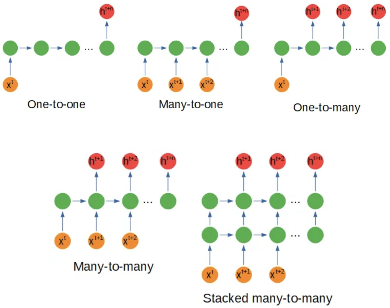
Sequential data in RNN (Recurrent Neural Network) refers to any type of data where the observations have a temporal or sequential relationship. This could include time series data, where each observation is dependent on the previous one, or sequence data, where the order of the observations is important. In RNNs, this type of data is processed through the recurrent connections in the network, allowing the model to maintain and update an internal state based on the information in the sequence. This makes RNNs particularly well suited for tasks such as language modeling, speech recognition, and time series forecasting. There are some variations to the neural network’s configuration based on the shape of the input or output which you can see in the following:
Order is not Important
The second limitation of traditional neural networks is that they can not remember the sequence of the data, or the order is not important to them. Let’s understand this problem with an example which is shown in this figure:

RNNs use feedback connections that allow information to be passed from one step of the sequence to the next, allowing the network to maintain and update an internal state that depends on the past input. This enables RNNs to capture and understand the dependencies and patterns in the sequence data, making them well suited for tasks such as natural language processing and time series analysis.
Cannot share parameters
In traditional Feedforward Neural Networks (MLPs), each input is processed independently and there is no mechanism for sharing parameters across different inputs in a sequence. For example, let’s take the sentence “what is your name? My name is Ryan”. In an MLP, each word would be treated as a separate input and would be processed through separate hidden layers. There is no way for the network to share information across words in the sequence, such as information about the relationship between words or about common features that occur across different parts of the sequence. In this case, “name”'s parameters should have been shared and so the neural network should have been able to determine that “name”'s words are dependent in this sentence.
In contrast, Recurrent Neural Networks (RNNs) have a hidden state that is updated at each time step, allowing the network to maintain information about the sequence and share parameters across different time steps. This makes RNNs well-suited for processing sequential data and for tasks such as sequence classification, language modeling, and machine translation
Therefore Recurrent Neural Networks (RNN), originally were designed to handle some of the shortcomings that traditional neural networks have when dealing with sequential data.
Recurrent Neural Networks
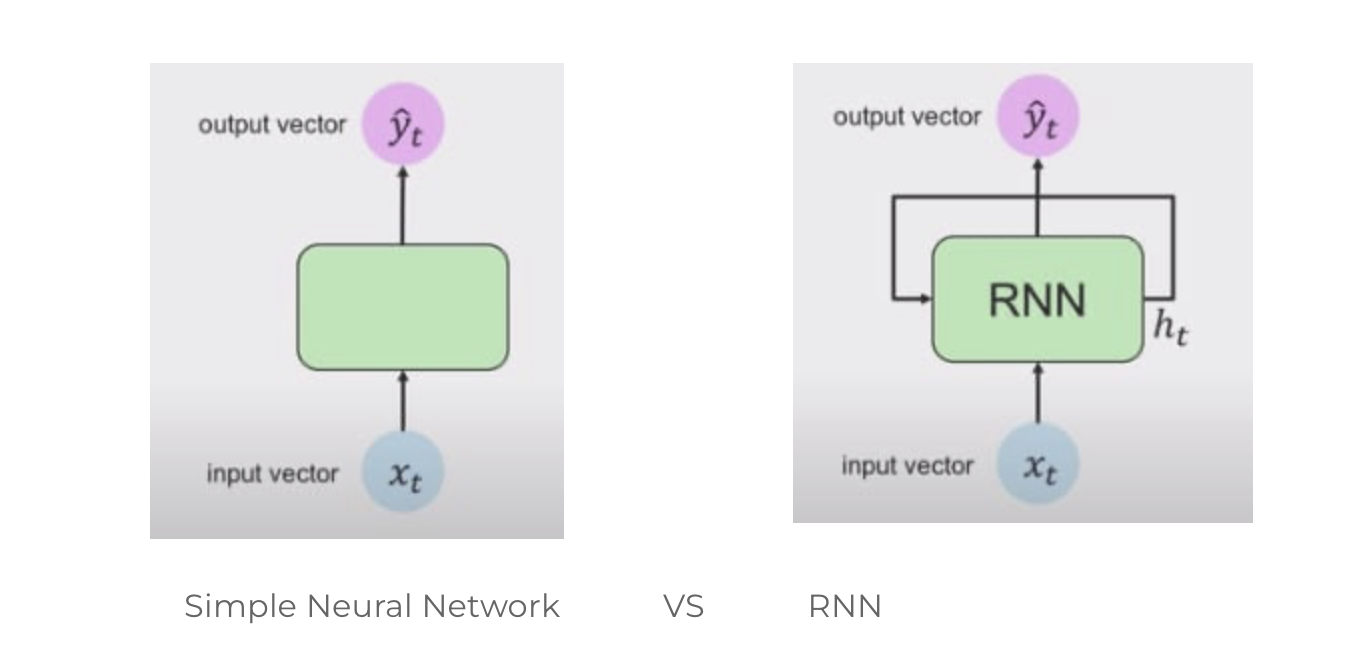
Here we can see that the Simple Neural Network is unidirectional, which means it has a single direction, whereas the RNN, has loops inside it to persist the information over timestamp t. This looping preserves the information over the sequence.
Now, let’s dig deeper to understand what is happening under the hood. An RNN consists of four different parts:
Linear part (Parameters: This includes the weights and biases of the input-to-hidden layer, the hidden-to-hidden layer, and the hidden-to-output layer.)
The hidden state is used to capture the information from the previous time steps, but this information is not relevant after the training process is finished. Therefore, resetting the hidden state parameters to zero ensures that the network starts with a clean slate for making predictions on new, unseen data.
The hidden state (also known as the context state)
you can think of the hidden state as representing the “memory” of the network, which is updated at each time step and used to produce the output.
Non-Linear part (Activation Function (ReLU))
For now we’re going to use the ReLU, however we’ll see that ReLU might not be the best pick for this network.
Fully connected (Output layer): Finally, you’ll have the output vector at the timestamp t.
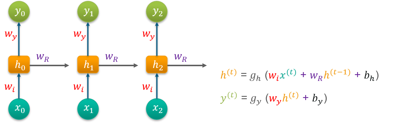
Recurrent Neural Network
In Recurrent Neural Networks (RNNs), the terms “input size”, “hidden size”, and “number of outputs” refer to the following:
Input size: Refers to the number of features in a single input sample. For example, if the input is a one-hot encoded word, the input size would be the number of unique words in the vocabulary.
Hidden size: Refers to the number of neurons in the hidden layer. The hidden state of the RNN at each time step is represented by this layer, which helps to capture information from the past time steps.
Number of outputs: Refers to the number of outputs generated by the RNN. This could be one output for a simple prediction problem, or multiple outputs for a multi-task prediction problem.
Note that these hyperparameters need to be set prior to training the RNN and their choice can affect the model’s performance.
The “input to hidden” weights are the connections or weights between the input layer and the hidden layer, and these connections allow the network to learn how to propagate information from the input to the hidden state.
The “hidden to output” weights are the connections or weights between the hidden layer and the output layer, and these connections allow the network to learn how to produce the final output based on the hidden state.
The forward pass is the process of computing the output for a given input sequence. The forward pass starts by initializing the hidden state of the RNN with a zero vector or some other randomly generated values.
In the forward pass we understood how the inputs and the hidden states interact with the weights and biases of the recurrent layers and how to use the information contained in the last hidden state to predict the next time step value.
RNNs use feedback connections that allow information to be passed from one step of the sequence to the next, allowing the network to maintain and update an internal state that depends on the past input. This enables RNNs to capture and understand the dependencies and patterns in the sequence data, making them well suited for tasks such as natural language processing and time series analysis.
The backward pass is just the application of the chain rule from the loss gradient with respect to the predictions until it becomes with respect to the parameters we want to optimize.
The hidden state is used to capture the information from the previous time steps, but this information is not relevant after the training process is finished. Therefore, resetting the hidden state to zero ensures that the network starts with a clean slate for making predictions on new, unseen data.
Pytorch Implementation
# import required libraries
import torch
import pandas as pd
import torch.nn as nn
import torch.optim as optim
import numpy as np
from torch.utils.data import DataLoader, TensorDataset
from sklearn import preprocessing
import matplotlib.pyplot as plt
from tqdm import tqdm
from sklearn.preprocessing import MinMaxScaler
To understand how should we prepare the data for RNN, we’ll use a simple dataset as a Timeseries Forecasting example. Below is the full sequence of values and their restructuring as a training and testing dataset.
$$ [10,20, 30, 40,50, 60, 70, 80, 90] \rightarrow
$$
Now, let’s separate the datasets into batches!
# Step 1: Load and Preprocess Data
df_array = pd.DataFrame(np.array([10, 20, 30, 40, 50, 60, 70, 80, 90]))
# Step 2: Normalize the Data
scaler = MinMaxScaler()
data_scaled = scaler.fit_transform(df_array)# Step 3: Split Data into Training and Testing Sets
train_size = int(len(data_scaled) * 0.8)
train_data = data_scaled[:train_size]
test_data = data_scaled[train_size:]
# Further split the training data into training and validation sets
train_valid_size = int(len(train_data) * 0.8)
train_data_final = train_data[:train_valid_size]
valid_data = train_data[train_valid_size:]
# Step 4: Prepare Data for RNN Input
def create_sequences_multivariate(data, n_timesteps, target_column_index):
X = []
y = []
for i in range(len(data) - n_timesteps):
seq_x = data[i:i + n_timesteps]
seq_y = data[i + n_timesteps, target_column_index]
X.append(seq_x)
y.append(seq_y)
return np.array(X), np.array(y)
n_timesteps = 1
n_features = data_scaled.shape[1]
target_column_index = 0 # 'Close' is the target column
# Create sequences for training, validation, and testing
X_train, y_train = create_sequences_multivariate(train_data_final, n_timesteps, target_column_index)
X_valid, y_valid = create_sequences_multivariate(valid_data, n_timesteps, target_column_index)
X_test, y_test = create_sequences_multivariate(test_data, n_timesteps, target_column_index)
# Convert to tensors
X_train = torch.tensor(X_train, dtype=torch.float32)
y_train = torch.tensor(y_train, dtype=torch.float32)
X_valid = torch.tensor(X_valid, dtype=torch.float32)
y_valid = torch.tensor(y_valid, dtype=torch.float32)
X_test = torch.tensor(X_test, dtype=torch.float32)
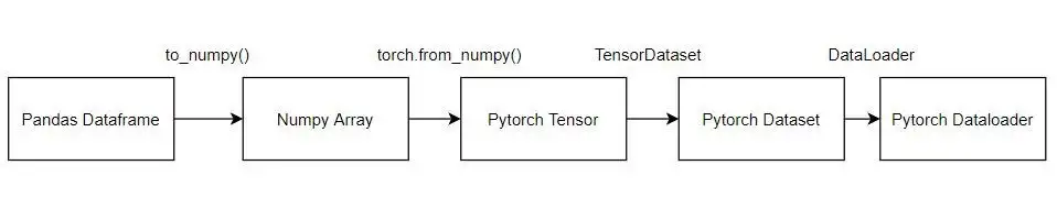
y_test = torch.tensor(y_test, dtype=torch.float32)We then have to prepare the dataset. We need the data as Pytorch tensors so that we can use that in our model which we will make. We use the dataloader so that we can extract the data in batches. This is especially helpful for large datasets.
# Create DataLoaders
train_dataset = TensorDataset(X_train, y_train)
valid_dataset = TensorDataset(X_valid, y_valid)
test_dataset = TensorDataset(X_test, y_test)

train_loader = DataLoader(train_dataset, batch_size=1, shuffle=False)
valid_loader = DataLoader(valid_dataset, batch_size=1, shuffle=False)
test_loader = DataLoader(test_dataset, batch_size=1, shuffle=False)
# Step 6: Build the RNN Model
# 1. Creating a FeedForwardNetwork
# 1.1 Structure (Architecture) of NN
class RNNModel(nn.Module):
def __init__(self, input_size, hidden_size=50, output_size=1):
super(RNNModel, self).__init__()
self.hidden_size = hidden_size
self.rnn = nn.RNN(input_size, hidden_size, batch_first=True)
self.fc = nn.Linear(hidden_size, output_size)
def forward(self, x):
out, h_n = self.rnn(x)
out = out[:, -1, :] # Take the output at the last time step
out = self.fc(out)
return out
model = RNNModel(input_size=n_features, hidden_size=50, output_size=1)
# Define loss function and optimizer
# 1.2 Loss Function
criterion = nn.MSELoss()
# 1.3 Optmization Approch
optimizer = optim.Adam(model.parameters())
# Step 7: Train the Model
device = torch.device('cuda' if torch.cuda.is_available() else 'cpu')
model.to(device)
num_epochs = 10
train_losses = []
valid_losses = []
for epoch in range(num_epochs):
model.train()
train_loss = 0
for inputs, targets in train_loader:
inputs = inputs.to(device)
targets = targets.to(device)
optimizer.zero_grad()
# 2. Forward Pass
outputs = model(inputs)
# 3. FeedForward Evaluation
loss = criterion(outputs.squeeze(), targets)
# 4. Backward Pass / Gradient Calculation
loss.backward()
# 5. Back Propagation / Update Weights
optimizer.step()
train_loss += loss.item() * inputs.size(0)
train_loss /= len(train_loader.dataset)
train_losses.append(train_loss)
# Evaluate on validation set
model.eval()
valid_loss = 0
with torch.no_grad():
for inputs, targets in valid_loader:
inputs = inputs.to(device)
targets = targets.to(device)
outputs = model(inputs)
loss = criterion(outputs.squeeze(), targets)
valid_loss += loss.item() * inputs.size(0)
valid_loss /= len(valid_loader.dataset)
valid_losses.append(valid_loss)
if (epoch + 1) % 2 == 0:
print(f'Epoch {epoch + 1}/{num_epochs}, Train Loss: {train_loss:.6f}, Valid Loss: {valid_loss:.6f}')
# Step 8: Evaluate the Model
# Evaluate on testing set
model.eval()
with torch.no_grad():
test_preds = model(X_test.to(device)).cpu().numpy()
test_actuals = y_test.numpy()
# # Step 9: Denormalize and Visualize Predictions
# # Since we have multiple features, we need to only inverse transform the target variable
# def denormalize(scaled_data, scaler, index):
# data = np.zeros((len(scaled_data), scaler.n_features_in_))
# data[:, index] = scaled_data[:, 0]
# data = scaler.inverse_transform(data)
# return data[:, index]
# # Denormalize the predictions and actuals
# test_preds_denorm = denormalize(test_preds, scaler, target_column_index)
# test_actuals_denorm = denormalize(test_actuals.reshape(-1, 1), scaler, target_column_index)
# # Plot predictions vs actuals for the test set
# plt.figure(figsize=(12, 6))
# plt.plot(test_actuals_denorm, label='Actual')
# plt.plot(test_preds_denorm, label='Predicted')
# plt.title('Predictions vs Actuals on Test Set')
# plt.xlabel('Index')
# plt.ylabel('TSLA Close Price')
# plt.legend()
# plt.show()
# # Step 10: Save and Load the Model
# # Save the model
# torch.save(model.state_dict(), 'tsla_rnn_model.pth')
# # Load the model
# loaded_model = RNNModel(input_size=n_features, hidden_size=50, output_size=1)
# loaded_model.load_state_dict(torch.load('tsla_rnn_model.pth'))
# loaded_model.to(device)
# loaded_model.eval()Epoch 2/10, Train Loss: 0.088995, Valid Loss: 0.420172
Epoch 4/10, Train Loss: 0.045331, Valid Loss: 0.299403
Epoch 6/10, Train Loss: 0.022258, Valid Loss: 0.211496
Epoch 8/10, Train Loss: 0.014069, Valid Loss: 0.154870
Epoch 10/10, Train Loss: 0.013384, Valid Loss: 0.124687
/home/sachi/venv/torch/lib/python3.13/site-packages/torch/cuda/__init__.py:180: UserWarning: CUDA initialization: The NVIDIA driver on your system is too old (found version 12070). Please update your GPU driver by downloading and installing a new version from the URL: http://www.nvidia.com/Download/index.aspx Alternatively, go to: https://pytorch.org to install a PyTorch version that has been compiled with your version of the CUDA driver. (Triggered internally at /pytorch/c10/cuda/CUDAFunctions.cpp:119.)
  return torch._C._cuda_getDeviceCount() > 0
/home/sachi/venv/torch/lib/python3.13/site-packages/torch/nn/modules/loss.py:626: UserWarning: Using a target size (torch.Size([1])) that is different to the input size (torch.Size([])). This will likely lead to incorrect results due to broadcasting. Please ensure they have the same size.
  return F.mse_loss(input, target, reduction=self.reduction)
# Combine the parameters of the RNN layer and linear layer
params = list(model.parameters())

# Print the number of parameters
print("Number of parameters:", sum(p.numel() for p in params))

# Print the shapes of the parameters
for name, param in model.named_parameters():
    print("Name: ", name)
    print("shape: ", param.shape)
    print("Weight: ", param.data)
Number of parameters: 2701
Name: rnn.weight_ih_l0
shape: torch.Size([50, 1])
Weight: tensor([[-0.0296],
[-0.1334],
[ 0.1249],
[-0.0653],
[ 0.0519],
[-0.1233],
[-0.0574],
[ 0.0800],
[-0.0950],
[-0.0262],
[ 0.0243],
[-0.1282],
[ 0.0146],
[ 0.0059],
[-0.0063],
[ 0.0922],
[-0.0888],
[ 0.0511],
[-0.0335],
[-0.0323],
[-0.0706],
[-0.0008],
[ 0.0012],
[-0.0480],
[-0.0317],
[-0.0223],
[-0.0544],
[ 0.1648],
[ 0.0674],
[-0.1647],
[ 0.0328],
[ 0.1145],
[-0.0114],
[-0.0362],
[-0.1179],
[-0.1096],
[-0.1020],
[ 0.0119],
[ 0.1545],
[ 0.0568],
[-0.0903],
[-0.0501],
[ 0.1444],
[ 0.1122],
[-0.0076],
[-0.0899],
[ 0.0505],
[ 0.1113],
[-0.1549],
[ 0.0288]])
Name: rnn.weight_hh_l0
shape: torch.Size([50, 50])
Weight: tensor([[-1.1871e-01, -6.8049e-03, -3.2712e-02, ..., -1.3660e-01,
-8.3000e-02, 1.1379e-01],
[ 1.2787e-01, 1.0897e-01, 8.3198e-03, ..., -1.0224e-01,
-2.8152e-02, 5.9048e-02],
[ 1.3770e-01, 1.3319e-01, 6.5657e-02, ..., 1.1642e-01,
-7.5670e-02, -5.3381e-02],
...,
[-5.2818e-05, 5.6223e-02, -3.7060e-02, ..., -7.8276e-02,
1.2691e-01, -1.0142e-01],
[ 9.9787e-03, 1.3792e-01, 1.3760e-01, ..., -3.5185e-02,
1.3774e-01, -9.2993e-04],
[ 7.3631e-02, -9.7294e-02, -1.1684e-01, ..., -1.4010e-01,
1.8867e-02, -1.3638e-01]])
Name: rnn.bias_ih_l0
shape: torch.Size([50])
Weight: tensor([ 0.0616, -0.0803, -0.0204, 0.1173, -0.0708, -0.0117, 0.0632, -0.0665,
-0.0504, 0.1515, 0.1063, 0.0703, -0.0725, 0.1581, 0.0824, -0.0768,
-0.1298, -0.0641, 0.0434, 0.1150, -0.0278, -0.1058, 0.0125, -0.1556,
-0.0788, 0.1217, -0.0871, 0.1261, 0.0330, -0.1249, 0.1051, 0.0563,
0.1399, 0.1034, -0.1587, 0.0964, -0.1360, 0.1137, -0.0082, 0.0743,
-0.0774, -0.0906, 0.1023, -0.0586, 0.1173, -0.0501, -0.0292, -0.1255,
0.0285, -0.0561])
Name: rnn.bias_hh_l0
shape: torch.Size([50])
Weight: tensor([ 0.0680, 0.0257, -0.0421, -0.1028, -0.1109, 0.0085, -0.0455, -0.0329,
0.0634, 0.0799, -0.1209, -0.1628, 0.0257, 0.0374, 0.0008, -0.0243,
0.1168, -0.0990, 0.0238, -0.0569, 0.0662, 0.0737, 0.0989, -0.1183,
-0.1433, -0.0092, 0.0590, 0.1652, 0.0388, -0.0507, 0.0126, 0.1116,
0.0991, 0.1074, -0.0123, 0.1558, 0.0249, -0.1523, 0.0204, 0.1044,
-0.0779, 0.0930, -0.0126, 0.0506, 0.0711, 0.0379, -0.0164, 0.0312,
0.0697, 0.0941])
Name: fc.weight
shape: torch.Size([1, 50])
Weight: tensor([[-0.1056, -0.1663, 0.0793, -0.0084, -0.0672, -0.0868, 0.0327, -0.0571,
-0.1011, 0.1492, -0.0087, -0.0816, 0.0909, 0.0314, 0.1353, -0.0004,
-0.0160, -0.0185, 0.0011, -0.0656, -0.0949, -0.0792, 0.1623, -0.1258,
-0.1183, 0.0664, -0.0786, 0.0850, -0.0424, -0.1015, 0.0717, 0.1594,
0.0373, 0.1507, -0.0980, 0.1434, -0.1041, -0.0325, 0.0774, -0.0163,
-0.0554, 0.0598, 0.0640, 0.1173, 0.0119, -0.0781, 0.1019, -0.1553,
-0.0402, -0.0702]])
Name: fc.bias
shape: torch.Size([1])
Weight: tensor([-0.0438])
| Layer | Description | Shape | Weight / Bias Values Explanation |
|---|---|---|---|
rnn.weight_ih_l0 | Input to Hidden Layer Weights | [50, 1] | Connects input feature to each of the 50 hidden units, influencing how input affects hidden activations. |
rnn.weight_hh_l0 | Hidden to Hidden Layer Weights | [50, 50] | Connects each hidden unit to every other hidden unit, capturing temporal dependencies across time steps. |
rnn.bias_ih_l0 | Input to Hidden Layer Biases | [50] | Adjusts the activation of each hidden unit to improve model flexibility for input transformations. |
rnn.bias_hh_l0 | Hidden to Hidden Layer Biases | [50] | Adjusts hidden state outputs after combining them with hidden-to-hidden transformations. |
fc.weight | Fully Connected Layer Weights | [1, 50] | Connects 50 hidden units to a single output, combining RNN hidden states into one final output. |
fc.bias | Fully Connected Layer Bias | [1] | Single bias term adjusting the output of the fully connected layer. |
Source
import plotly.graph_objects as go
import numpy as np

# ============================================================
# RNN ARCHITECTURE VISUALIZATION
# ============================================================

INPUT_SIZE = 1
HIDDEN_SIZE = 50
OUTPUT_SIZE = 1

fig = go.Figure()

# ------------------------------------------------------------
# NODE POSITIONS
# ------------------------------------------------------------

x_input = 0
x_hidden = 6
x_output = 12

# vertically center hidden layer
hidden_y = np.linspace(-25, 25, HIDDEN_SIZE)

# input/output centered
input_y = [0]
output_y = [0]

# ------------------------------------------------------------
# DRAW INPUT NODE
# ------------------------------------------------------------

fig.add_trace(
    go.Scatter(
        x=[x_input],
        y=input_y,
        mode="markers+text",
        marker=dict(size=28),
        text=["Input\n(1 feature)"],
        textposition="bottom center",
        name="Input Layer",
        hovertemplate=(
            "<b>Input Layer</b><br>"
            "Shape: [1]<br>"
            "Single time-series feature input"
            "<extra></extra>"
        )
    )
)

# ------------------------------------------------------------
# DRAW HIDDEN NODES
# ------------------------------------------------------------

fig.add_trace(
    go.Scatter(
        x=[x_hidden] * HIDDEN_SIZE,
        y=hidden_y,
        mode="markers",
        marker=dict(size=12),
        name="Hidden Layer",
        text=[
            (
                f"<b>Hidden Unit {i}</b><br>"
                f"Receives:<br>"
                "- Input weights from rnn.weight_ih_l0 [50,1]<br>"
                "- Recurrent weights from rnn.weight_hh_l0 [50,50]<br>"
                "- Biases from rnn.bias_ih_l0 and rnn.bias_hh_l0"
            )
            for i in range(HIDDEN_SIZE)
        ],
        hoverinfo="text"
    )
)

# ------------------------------------------------------------
# DRAW OUTPUT NODE
# ------------------------------------------------------------

fig.add_trace(
    go.Scatter(
        x=[x_output],
        y=output_y,
        mode="markers+text",
        marker=dict(size=28),
        text=["Output\n(1 value)"],
        textposition="bottom center",
        name="Output Layer",
        hovertemplate=(
            "<b>Output Layer</b><br>"
            "Shape: [1]<br>"
            "Receives weighted combination<br>"
            "from all 50 hidden units via fc.weight [1,50]"
            "<extra></extra>"
        )
    )
)

# ============================================================
# EDGES
# ============================================================

edge_x = []
edge_y = []

# ------------------------------------------------------------
# INPUT -> HIDDEN
# rnn.weight_ih_l0 [50,1]
# ------------------------------------------------------------

for hy in hidden_y:
    edge_x.extend([x_input, x_hidden, None])
    edge_y.extend([0, hy, None])

fig.add_trace(
    go.Scatter(
        x=edge_x,
        y=edge_y,
        mode="lines",
        line=dict(width=1),
        opacity=0.35,
        hoverinfo="skip",
        name="Input -> Hidden"
    )
)

# ------------------------------------------------------------
# HIDDEN -> OUTPUT
# fc.weight [1,50]
# ------------------------------------------------------------

edge_x = []
edge_y = []

for hy in hidden_y:
    edge_x.extend([x_hidden, x_output, None])
    edge_y.extend([hy, 0, None])

fig.add_trace(
    go.Scatter(
        x=edge_x,
        y=edge_y,
        mode="lines",
        line=dict(width=1),
        opacity=0.35,
        hoverinfo="skip",
        name="Hidden -> Output"
    )
)

# ------------------------------------------------------------
# RECURRENT CONNECTIONS
# rnn.weight_hh_l0 [50,50]
# ------------------------------------------------------------

# Instead of drawing all 2500 edges (too messy),
# draw representative recurrent loops.

loop_x = []
loop_y = []

for hy in hidden_y[::5]:  # every 5th node
    theta = np.linspace(0, 2*np.pi, 40)
    radius = 0.45

    xs = x_hidden + radius * np.cos(theta)
    ys = hy + radius * np.sin(theta)

    loop_x.extend(xs.tolist() + [None])
    loop_y.extend(ys.tolist() + [None])

fig.add_trace(
    go.Scatter(
        x=loop_x,
        y=loop_y,
        mode="lines",
        line=dict(width=2, dash="dot"),
        name="Recurrent Connections",
        hovertemplate=(
            "<b>rnn.weight_hh_l0</b><br>"
            "Shape: [50,50]<br>"
            "Each hidden unit connects to all hidden units<br>"
            "across time steps"
            "<extra></extra>"
        )
    )
)

# ============================================================
# ANNOTATIONS
# ============================================================

fig.add_annotation(
    x=3,
    y=30,
    text="rnn.weight_ih_l0 [50,1]",
    showarrow=False,
    font=dict(size=13)
)

fig.add_annotation(
    x=9,
    y=30,
    text="fc.weight [1,50]",
    showarrow=False,
    font=dict(size=13)
)

fig.add_annotation(
    x=6,
    y=-32,
    text="rnn.weight_hh_l0 [50,50]",
    showarrow=False,
    font=dict(size=13)
)

# ============================================================
# LAYOUT
# ============================================================

fig.update_layout(
    title="RNN Neural Network Architecture",
    width=1400,
    height=900,
    dragmode="zoom",
    hovermode="closest",
    showlegend=True,
    template="plotly_white",
    xaxis=dict(
        visible=False
    ),
    yaxis=dict(
        visible=False
    )
)

# ------------------------------------------------------------
# RENDER
# ------------------------------------------------------------

fig.show()RNN for Time Series Forecasting
# Import necessary libraries
import pandas as pd
import numpy as np
import yfinance as yf
import torch
import torch.nn as nn
import torch.optim as optim
from torch.utils.data import TensorDataset, DataLoader
from sklearn.preprocessing import MinMaxScaler
import matplotlib.pyplot as plt

# Step 1: Load and Preprocess Data
# Load dataset
end_date = pd.Timestamp.today()
start_date = end_date - pd.DateOffset(years=5)  # Last 5 years
df = yf.download('AAPL', start=start_date, end=end_date)
df = df[['Close']]
df = df.sort_index()

# Step 2: Create Lag and Rolling Features
df['lag_5'] = df['Close'].shift(5)
df['rolling_mean_10'] = df['Close'].rolling(window=10).mean()
df['rolling_sd_10'] = df['Close'].rolling(window=10).std()
# df['rolling_diff_10'] = df['Close'] - df['rolling_mean_10']
df.dropna(inplace=True)

# Step 3: Normalize the Data
scaler = MinMaxScaler()
data_scaled = scaler.fit_transform(df)
[*********************100%***********************] 1 of 1 completed
# Step 4: Split Data into Training and Testing Sets

SEQUENCE_LENGTH = 20

X, y = [], []

for i in range(SEQUENCE_LENGTH, len(data_scaled)):
    X.append(data_scaled[i-SEQUENCE_LENGTH:i])
    y.append(data_scaled[i, 0])  # Close price only

X = np.array(X)
y = np.array(y)
split_index = int(len(X) * 0.8)
X_train = X[:split_index]
X_test = X[split_index:]
y_train = y[:split_index]
y_test = y[split_index:]X_train = torch.tensor(X_train, dtype=torch.float32)
y_train = torch.tensor(y_train, dtype=torch.float32).unsqueeze(-1)
X_test = torch.tensor(X_test, dtype=torch.float32)
y_test = torch.tensor(y_test, dtype=torch.float32).unsqueeze(-1)train_dataset = TensorDataset(X_train, y_train)
train_loader = DataLoader(train_dataset, batch_size=32, shuffle=True)# Step 5: Initialize the Model
input_size = X_train.shape[2]
model = RNNModel(input_size=input_size)
criterion = nn.MSELoss()
optimizer = optim.Adam(model.parameters(), lr=0.001)# Step 6: Train the Model
epochs = 50
for epoch in range(epochs):
model.train()
epoch_loss = 0
for batch_X, batch_y in train_loader:
optimizer.zero_grad()
preds = model(batch_X)
loss = criterion(preds, batch_y)
loss.backward()
optimizer.step()
epoch_loss += loss.item()
if epoch % 10 == 0:
print(f"Epoch {epoch}: Loss = {epoch_loss/len(train_loader):.6f}")Epoch 0: Loss = 0.045053
Epoch 10: Loss = 0.000976
Epoch 20: Loss = 0.000726
Epoch 30: Loss = 0.000591
Epoch 40: Loss = 0.000603
# Step 7: Make Predictions on the Test Set

model.eval()

with torch.no_grad():
    test_preds = model(X_test)

test_preds = test_preds.squeeze().numpy()
y_test_np = y_test.squeeze().numpy()
Source
dummy_pred = np.zeros((len(test_preds), df.shape[1]))
dummy_true = np.zeros((len(y_test_np), df.shape[1]))

dummy_pred[:, 0] = test_preds
dummy_true[:, 0] = y_test_np

pred_prices = scaler.inverse_transform(dummy_pred)[:, 0]
true_prices = scaler.inverse_transform(dummy_true)[:, 0]
Source
import matplotlib.pyplot as plt
import numpy as np

# ============================================================
# 1. Reconstruct FULL price series (from scaled y)
# ============================================================

dummy_full = np.zeros((len(y), df.shape[1]))
dummy_full[:, 0] = y

full_true_prices = scaler.inverse_transform(dummy_full)[:, 0]

# ============================================================
# 2. Align train/test split (IMPORTANT: y is sequence-based)
# ============================================================

train_true = full_true_prices[:split_index]
test_true = full_true_prices[split_index:]

# ============================================================
# 3. Ensure predictions align
# (pred_prices already corresponds to test_true)
# ============================================================

# safety check
pred_prices = np.array(pred_prices).reshape(-1)

# trim mismatch if needed
min_len = min(len(test_true), len(pred_prices))
test_true = test_true[:min_len]
pred_prices = pred_prices[:min_len]

# ============================================================
# 4. Context window BEFORE test start
# ============================================================

context_window = 100
context = train_true[-context_window:]

# ============================================================
# 5. X-axis construction
# ============================================================

context_x = np.arange(len(context))
test_x = np.arange(len(context), len(context) + len(test_true))

# ============================================================
# 6. Plot
# ============================================================

plt.figure(figsize=(14,6))

# historical context
plt.plot(context_x, context, label="Context (Train History)", color="gray")

# true test values
plt.plot(test_x, test_true, label="Actual Price")

# predictions
plt.plot(test_x, pred_prices, label="Predicted Price")

plt.axvline(x=len(context), linestyle="--", color="black", alpha=0.5)

plt.title("AAPL RNN Prediction with Context")
plt.xlabel("Time")
plt.ylabel("Price")

plt.legend()
plt.grid(True)
plt.show()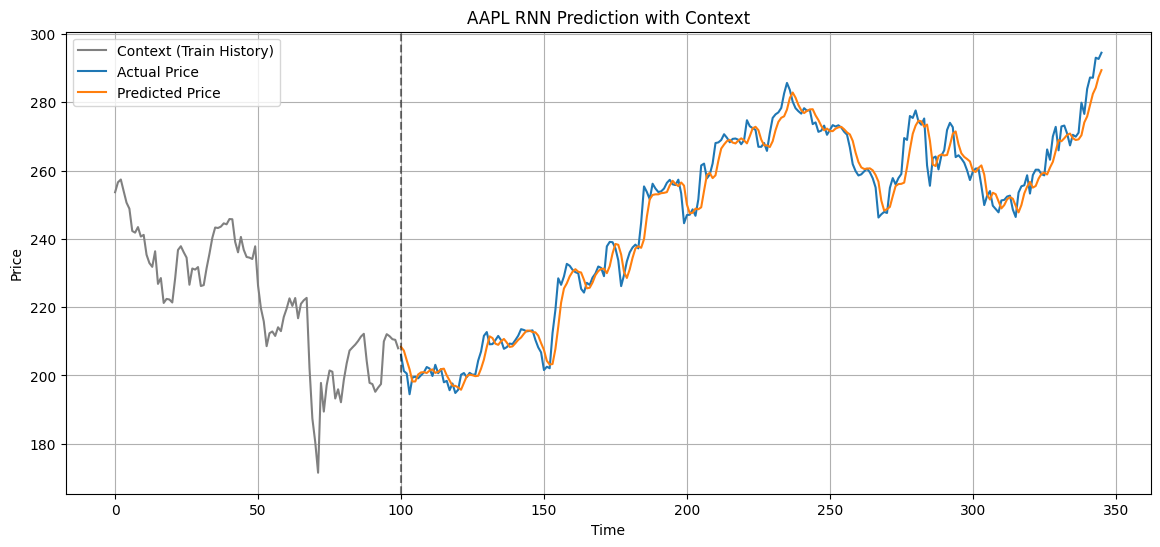
from sklearn.metrics import mean_absolute_error, mean_squared_error, r2_score
import numpy as np

mae = mean_absolute_error(true_prices, pred_prices)
rmse = np.sqrt(mean_squared_error(true_prices, pred_prices))
r2 = r2_score(true_prices, pred_prices)

print("MAE:", mae)
print("RMSE:", rmse)
print("R²:", r2)
MAE: 3.203765898779607
RMSE: 4.379834606934193
R²: 0.9732090806261626
Long Short Term Memory
One of the main problems of classical RNNs is so-called vanishing gradients problem. Because RNNs are trained end-to-end in one back-propagation pass, it is having hard times propagating error to the first layers of the network, and thus the network cannot learn relationships between distant tokens. One of the ways to avoid this problem is to introduce explicit state management by using so called gates. There are two most known architectures of this kind: Long Short Term Memory (LSTM) and Gated Relay Unit (GRU).

Given the input sequence of tokens , RNN creates a sequence of neural network blocks, and trains this sequence end-to-end using back propagation. Each network block takes a pair as an input, and produces as a result. Final state or output goes into a linear classifier to produce the result. All network blocks share the same weights, and are trained end-to-end using one back propagation pass.
Because state vectors are passed through the network, it is able to learn the sequential dependencies between words. For example, when the word not appears somewhere in the sequence, it can learn to negate certain elements within the state vector, resulting in negation.
from datasets import load_dataset
dataset = load_dataset("bentrevett/multi30k")
/home/sachi/venv/torch/lib/python3.13/site-packages/tqdm/auto.py:21: TqdmWarning: IProgress not found. Please update jupyter and ipywidgets. See https://ipywidgets.readthedocs.io/en/stable/user_install.html
from .autonotebook import tqdm as notebook_tqdm
Warning: You are sending unauthenticated requests to the HF Hub. Please set a HF_TOKEN to enable higher rate limits and faster downloads.
Generating train split: 100%|██████████| 29000/29000 [00:00<00:00, 518831.33 examples/s]
Generating validation split: 100%|██████████| 1014/1014 [00:00<00:00, 285227.30 examples/s]
Generating test split: 100%|██████████| 1000/1000 [00:00<00:00, 344190.38 examples/s]
dataset["train"][0]{'en': 'Two young, White males are outside near many bushes.',
'de': 'Zwei junge weiße Männer sind im Freien in der Nähe vieler Büsche.'}Source
from collections import Counter
import torch
import numpy as np

def tokenize(text):
    return text.lower().strip().split()

counter = Counter()

for item in dataset["train"]:
    counter.update(tokenize(item["en"]))
    counter.update(tokenize(item["de"]))

word2idx = {
    "<pad>": 0,
    "<sos>": 1,
    "<eos>": 2,
    "<unk>": 3
}

for w in counter:
    word2idx[w] = len(word2idx)

idx2word = {i: w for w, i in word2idx.items()}
vocab_size = len(word2idx)

def encode(text):
    return [word2idx.get(w, 3) for w in tokenize(text)]

MAX_LEN = 20

def pad(seq):
    return seq + [0] * (MAX_LEN - len(seq))
from torch.utils.data import Dataset, DataLoader
import torch
class TranslationDataset(Dataset):
def __init__(self, data):
self.data = data
def __len__(self):
return len(self.data)
def __getitem__(self, idx):
item = self.data[idx]
src = pad(encode(item["en"])[:MAX_LEN])
tgt = pad(encode(item["de"])[:MAX_LEN])
return torch.tensor(src), torch.tensor(tgt)class Encoder(nn.Module):
def __init__(self, vocab_size, emb=128, hidden=256):
super().__init__()
self.embedding = nn.Embedding(vocab_size, emb)
self.lstm = nn.LSTM(emb, hidden, batch_first=True)
def forward(self, x):
x = self.embedding(x)
_, (h, c) = self.lstm(x)
return h, cSource
class Decoder(nn.Module):
    def __init__(self, vocab_size, emb=128, hidden=256, rnn_hidden=128):
        super().__init__()

        self.embedding = nn.Embedding(vocab_size, emb)

        # LSTM layer (sequence modeling)
        self.lstm = nn.LSTM(emb, hidden, batch_first=True)

        # RNN refinement layer
        self.rnn = nn.RNN(hidden, rnn_hidden, batch_first=True)

        self.fc = nn.Linear(rnn_hidden, vocab_size)

    def forward(self, x, h, c):
        x = self.embedding(x)

        lstm_out, (h, c) = self.lstm(x, (h, c))

        rnn_out, _ = self.rnn(lstm_out)

        out = self.fc(rnn_out)

        return out, h, c
class Seq2Seq(nn.Module):
def __init__(self, vocab_size):
super().__init__()
self.encoder = Encoder(vocab_size)
self.decoder = Decoder(vocab_size)
def forward(self, src, tgt):
h, c = self.encoder(src)
out, _, _ = self.decoder(tgt, h, c)
return outtrain_data = TranslationDataset(dataset["train"])
train_loader = DataLoader(train_data, batch_size=64, shuffle=True)model = Seq2Seq(vocab_size)
criterion = nn.CrossEntropyLoss(ignore_index=0)
optimizer = torch.optim.Adam(model.parameters(), lr=0.001)device = torch.device("cuda" if torch.cuda.is_available() else "cpu")
model = model.to(device)
for epoch in range(3):
total_loss = 0
for src, tgt in train_loader:
src = src.to(device)
tgt = tgt.to(device)
tgt_input = torch.cat([
torch.full((tgt.size(0), 1), 1).to(device), # <sos>
tgt
], dim=1)
tgt_output = torch.cat([
tgt,
torch.full((tgt.size(0), 1), 2).to(device) # <eos>
], dim=1)
optimizer.zero_grad()
output = model(src, tgt_input)
loss = criterion(
output.reshape(-1, vocab_size),
tgt_output.reshape(-1)
)
loss.backward()
optimizer.step()
total_loss += loss.item()
print(f"Epoch {epoch}: Loss {total_loss:.4f}")