Lecture 20 - (07/05/26)
Today’s Topics:
Computer Vision
Convolutional Neural Networks
# Import PyTorch
import torch
from torch import nn

# Import torchvision
import torchvision
from torchvision import datasets
from torchvision.transforms import ToTensor

# Import matplotlib for visualization
import matplotlib.pyplot as plt

# Check versions
print(f"PyTorch version: {torch.__version__}\ntorchvision version: {torchvision.__version__}")
PyTorch version: 2.11.0+cu130
torchvision version: 0.26.0+cu130
Computer Vision
Fashion MNIST
The original MNIST dataset contains thousands of examples of handwritten digits (from 0 to 9) and was used to build computer vision models to identify numbers for postal services.
FashionMNIST, made by Zalando Research, is a similar setup, except it contains grayscale images of 10 different kinds of clothing.
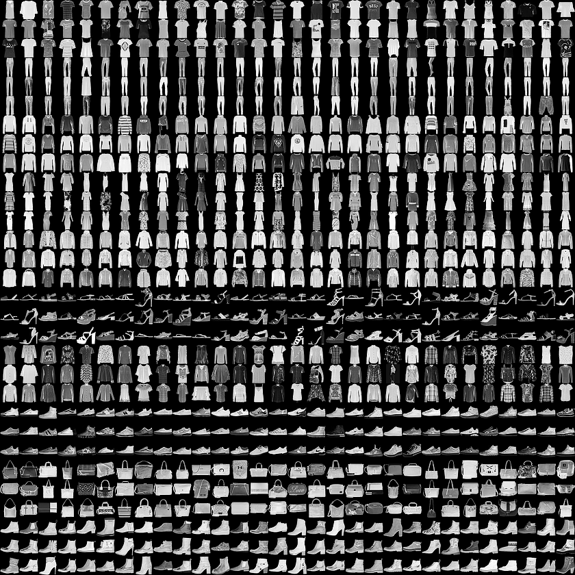
Let’s build a computer vision neural network to identify the different styles of clothing in these images.
# Setup training data
train_data = datasets.FashionMNIST(
    root="data", # where to download data to?
    train=True, # get training data
    download=True, # download data if it doesn't exist on disk
    transform=ToTensor(), # images come as PIL format, we want to turn into Torch tensors
    target_transform=None # you can transform labels as well
)

# Setup testing data
test_data = datasets.FashionMNIST(
    root="data",
    train=False, # get test data
    download=True,
    transform=ToTensor()
)
image, label = train_data[0]
image.shapetorch.Size([1, 28, 28])The shape of the image tensor is [1, 28, 28] or more specifically:
1 Color Channel
28 Height
28 Width
Having 1 color channel means the image is greyscale.
Note: Some datasets use CHW order, and others use HWC, it generally depends on which library you are using.
You might also see NCHW or NHWC where n stands for number of images. PyTorch generally accepts NCHW as the default and claims that it performs better and is best practice.
# How many samples are there?
len(train_data.data), len(train_data.targets), len(test_data.data), len(test_data.targets)
(60000, 60000, 10000, 10000)So we’ve got 60,000 training samples and 10,000 testing samples.
What classes are there?
# See classes
class_names = train_data.classes
class_names
['T-shirt/top',
'Trouser',
'Pullover',
'Dress',
'Coat',
'Sandal',
'Shirt',
'Sneaker',
'Bag',
'Ankle boot']Because we’re working with 10 different classes, it means our problem is multi-class classification.
Visualizing the Data
import matplotlib.pyplot as plt
image, label = train_data[0]
print(f"Image shape: {image.shape}")
plt.imshow(image.squeeze()) # image shape is [1, 28, 28] (colour channels, height, width)
plt.title(label);
Image shape: torch.Size([1, 28, 28])
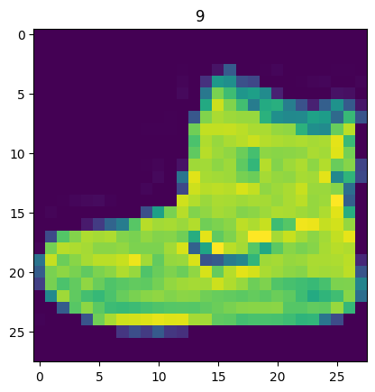
We can turn the image into grayscale using the cmap parameter of plt.imshow().
plt.imshow(image.squeeze(), cmap="gray")
plt.title(class_names[label]);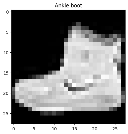
Let’s view a few more.
# Plot more images
torch.manual_seed(42)
fig = plt.figure(figsize=(9, 9))
rows, cols = 4, 4
for i in range(1, rows * cols + 1):
    random_idx = torch.randint(0, len(train_data), size=[1]).item()
    img, label = train_data[random_idx]
    fig.add_subplot(rows, cols, i)
    plt.imshow(img.squeeze(), cmap="gray")
    plt.title(class_names[label])
    plt.axis(False);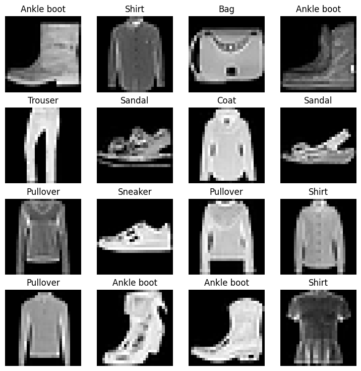
Now we’ve got a dataset ready to go. The next step is to prepare it with a DataLoader.
The DataLoader turns a large dataset into a Python iterable of smaller chunks. These smaller chunks are called batches or mini-batches and can be set by the batch_size parameter.
The reason we have to do this is because while it would be nice to do the forward pass and backwards pass across all of your data, realistically we have to reak it into smaller batches.
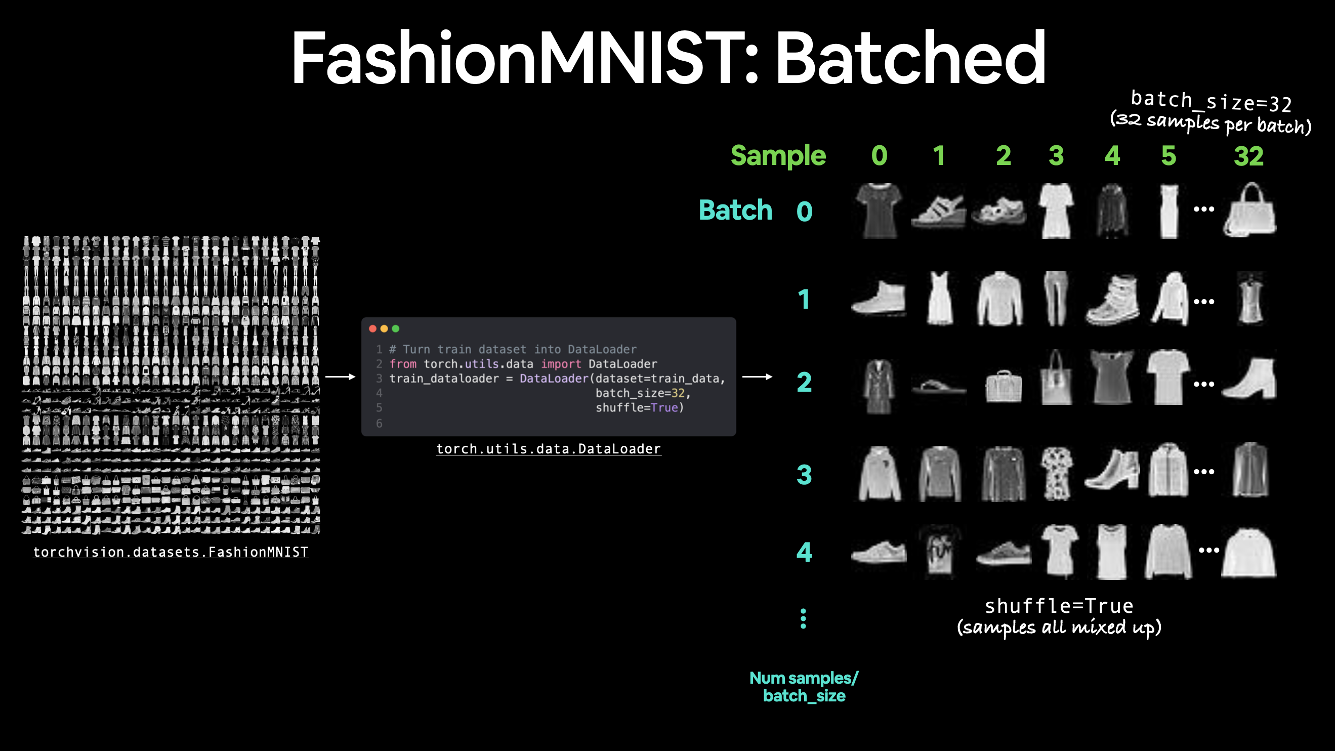
from torch.utils.data import DataLoader

# Setup the batch size hyperparameter
BATCH_SIZE = 32

# Turn datasets into iterables (batches)
train_dataloader = DataLoader(train_data, # dataset to turn into iterable
    batch_size=BATCH_SIZE, # how many samples per batch?
    shuffle=True # shuffle data every epoch?
)

test_dataloader = DataLoader(test_data,
    batch_size=BATCH_SIZE,
    shuffle=False # don't necessarily have to shuffle the testing data
)

# Let's check out what we've created
print(f"Dataloaders: {train_dataloader, test_dataloader}")
print(f"Length of train dataloader: {len(train_dataloader)} batches of {BATCH_SIZE}")
print(f"Length of test dataloader: {len(test_dataloader)} batches of {BATCH_SIZE}")
Dataloaders: (<torch.utils.data.dataloader.DataLoader object at 0x7c1d33d22ba0>, <torch.utils.data.dataloader.DataLoader object at 0x7c1d225b4a50>)
Length of train dataloader: 1875 batches of 32
Length of test dataloader: 313 batches of 32
# Check out what's inside the training dataloader
train_features_batch, train_labels_batch = next(iter(train_dataloader))
train_features_batch.shape, train_labels_batch.shape
(torch.Size([32, 1, 28, 28]), torch.Size([32]))And we can see that the data remains unchanged by checking a single sample.
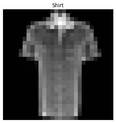
# Show a sample
torch.manual_seed(42)
random_idx = torch.randint(0, len(train_features_batch), size=[1]).item()
img, label = train_features_batch[random_idx], train_labels_batch[random_idx]
plt.imshow(img.squeeze(), cmap="gray")
plt.title(class_names[label])
plt.axis("Off");
print(f"Image size: {img.shape}")
print(f"Label: {label}, label size: {label.shape}")
Image size: torch.Size([1, 28, 28])
Label: 6, label size: torch.Size([])
Building the Model
Time to build a baseline model by subclassing nn.Module.
Our baseline will consist of two nn.Linear() layers.
Because we’re working with image data, we don’t want to deal with the overhead of a 2D Tensor, so we start by flattening it into a single vector. We can do this by inputting the image into a nn.Flatten() layer.
# Create a flatten layer
flatten_model = nn.Flatten() # all nn modules function as a model (can do a forward pass)

# Get a single sample
x = train_features_batch[0]

# Flatten the sample
output = flatten_model(x) # perform forward pass

# Print out what happened
print(f"Shape before flattening: {x.shape} -> [color_channels, height, width]")
print(f"Shape after flattening: {output.shape} -> [color_channels, height*width]")
Shape before flattening: torch.Size([1, 28, 28]) -> [color_channels, height, width]
Shape after flattening: torch.Size([1, 784]) -> [color_channels, height*width]
Let’s create our first model using nn.Flatten() as the first layer.
from torch import nn
class FashionMNISTModelV0(nn.Module):
    def __init__(self, input_shape: int, hidden_units: int, output_shape: int):
        super().__init__()
        self.layer_stack = nn.Sequential(
            nn.Flatten(), # neural networks like their inputs in vector form
            nn.Linear(in_features=input_shape, out_features=hidden_units), # in_features = number of features in a data sample (784 pixels)
            nn.Linear(in_features=hidden_units, out_features=output_shape)
        )

    def forward(self, x):
        return self.layer_stack(x)
We’ve got a baseline model class we can use, now let’s instantiate a model.
We’ll need to set the following parameters:
input_shape=784- this is how many features you’ve got going in the model, in our case, it’s one for every pixel in the target image (28 pixels high by 28 pixels wide = 784 features).hidden_units=10- number of units/neurons in the hidden layer(s), this number could be whatever you want but to keep the model small we’ll start with10.output_shape=len(class_names)- since we’re working with a multi-class classification problem, we need an output neuron per class in our dataset.
torch.manual_seed(42)

# Need to setup model with input parameters
model_0 = FashionMNISTModelV0(input_shape=784, # one for every pixel (28x28)
    hidden_units=10, # how many units in the hidden layer
    output_shape=len(class_names) # one for every class
)
model_0.to("cpu") # keep model on CPU
FashionMNISTModelV0(
(layer_stack): Sequential(
(0): Flatten(start_dim=1, end_dim=-1)
(1): Linear(in_features=784, out_features=10, bias=True)
(2): Linear(in_features=10, out_features=10, bias=True)
)
)Source
# Calculate accuracy (a classification metric)
def accuracy_fn(y_true, y_pred):
    """Calculates accuracy between truth labels and predictions.

    Args:
        y_true (torch.Tensor): Truth labels for predictions.
        y_pred (torch.Tensor): Predictions to be compared to predictions.

    Returns:
        [torch.float]: Accuracy value between y_true and y_pred, e.g. 78.45
    """
    correct = torch.eq(y_true, y_pred).sum().item()
    acc = (correct / len(y_pred)) * 100
    return acc
# Setup loss function and optimizer
loss_fn = nn.CrossEntropyLoss() # this is also called "criterion"/"cost function" in some places
optimizer = torch.optim.SGD(params=model_0.parameters(), lr=0.1)Source
from timeit import default_timer as timer
def print_train_time(start: float, end: float, device: torch.device = None):
    """Prints difference between start and end time.

    Args:
        start (float): Start time of computation (preferred in timeit format).
        end (float): End time of computation.
        device ([type], optional): Device that compute is running on. Defaults to None.

    Returns:
        float: time between start and end in seconds (higher is longer).
    """
    total_time = end - start
    print(f"Train time on {device}: {total_time:.3f} seconds")
    return total_time
Training the model
Let’s now create a training loop and a testing loop to train and evaluate our model.
Since we’re computing on batches of data, our loss and evaluation metrics will be calculated per batch rather than across the whole dataset. This means we’ll have to divide our loss and accuracy values by the number of batches in each dataset’s respective dataloader.
Loop through epochs.
Loop through training batches, perform training steps, calculate the train loss per batch.
Loop through testing batches, perform testing steps, calculate the test loss per batch.
Print out what’s happening.
# Import tqdm for progress bar
from tqdm.auto import tqdm

# Set the seed and start the timer
torch.manual_seed(42)
train_time_start = timer()

# Set the number of epochs (we'll keep this small for faster training times)
epochs = 3

# Create training and testing loop
for epoch in tqdm(range(epochs)):
    print(f"Epoch: {epoch}\n-------")
    ### Training
    train_loss = 0
    # Add a loop to loop through training batches
    for batch, (X, y) in enumerate(train_dataloader):
        model_0.train()
        # 1. Forward pass
        y_pred = model_0(X)

        # 2. Calculate loss (per batch)
        loss = loss_fn(y_pred, y)
        train_loss += loss # accumulatively add up the loss per epoch

        # 3. Optimizer zero grad
        optimizer.zero_grad()

        # 4. Loss backward
        loss.backward()

        # 5. Optimizer step
        optimizer.step()

        # Print out how many samples have been seen
        if batch % 400 == 0:
            print(f"Looked at {batch * len(X)}/{len(train_dataloader.dataset)} samples")

    # Divide total train loss by length of train dataloader (average loss per batch per epoch)
    train_loss /= len(train_dataloader)

    ### Testing
    # Setup variables for accumulatively adding up loss and accuracy
    test_loss, test_acc = 0, 0
    model_0.eval()
    with torch.inference_mode():
        for X, y in test_dataloader:
            # 1. Forward pass
            test_pred = model_0(X)

            # 2. Calculate loss (accumulatively)
            test_loss += loss_fn(test_pred, y) # accumulatively add up the loss per epoch

            # 3. Calculate accuracy (preds need to be same as y_true)
            test_acc += accuracy_fn(y_true=y, y_pred=test_pred.argmax(dim=1))

        # Calculations on test metrics need to happen inside torch.inference_mode()
        # Divide total test loss by length of test dataloader (per batch)
        test_loss /= len(test_dataloader)

        # Divide total accuracy by length of test dataloader (per batch)
        test_acc /= len(test_dataloader)

    ## Print out what's happening
    print(f"\nTrain loss: {train_loss:.5f} | Test loss: {test_loss:.5f}, Test acc: {test_acc:.2f}%\n")

# Calculate training time
train_time_end = timer()
total_train_time_model_0 = print_train_time(start=train_time_start,
                                           end=train_time_end,
                                           device=str(next(model_0.parameters()).device))
/home/sachi/venv/torch/lib/python3.13/site-packages/tqdm/auto.py:21: TqdmWarning: IProgress not found. Please update jupyter and ipywidgets. See https://ipywidgets.readthedocs.io/en/stable/user_install.html
from .autonotebook import tqdm as notebook_tqdm
0%| | 0/3 [00:00<?, ?it/s]Epoch: 0
-------
Looked at 0/60000 samples
/home/sachi/venv/torch/lib/python3.13/site-packages/torch/autograd/graph.py:869: UserWarning: CUDA initialization: The NVIDIA driver on your system is too old (found version 12070). Please update your GPU driver by downloading and installing a new version from the URL: http://www.nvidia.com/Download/index.aspx Alternatively, go to: https://pytorch.org to install a PyTorch version that has been compiled with your version of the CUDA driver. (Triggered internally at /pytorch/c10/cuda/CUDAFunctions.cpp:119.)
  return Variable._execution_engine.run_backward(  # Calls into the C++ engine to run the backward pass
Looked at 12800/60000 samples
Looked at 25600/60000 samples
Looked at 38400/60000 samples
Looked at 51200/60000 samples
33%|███▎ | 1/3 [00:06<00:12, 6.38s/it]
Train loss: 0.59039 | Test loss: 0.50954, Test acc: 82.04%

Epoch: 1
-------
Looked at 0/60000 samples
Looked at 12800/60000 samples
Looked at 25600/60000 samples
Looked at 38400/60000 samples
Looked at 51200/60000 samples
67%|██████▋ | 2/3 [00:13<00:06, 6.58s/it]
Train loss: 0.47633 | Test loss: 0.47989, Test acc: 83.20%

Epoch: 2
-------
Looked at 0/60000 samples
Looked at 12800/60000 samples
Looked at 25600/60000 samples
Looked at 38400/60000 samples
Looked at 51200/60000 samples
100%|██████████| 3/3 [00:19<00:00, 6.60s/it]
Train loss: 0.45503 | Test loss: 0.47664, Test acc: 83.43%

Train time on cpu: 19.794 seconds
Since we’re going to be building a few models, it’s a good idea to write some code to evaluate them all in similar ways.
Namely, let’s create a function that takes in a trained model, a DataLoader, a loss function and an accuracy function.
Source
torch.manual_seed(42)
def eval_model(model: torch.nn.Module,
               data_loader: torch.utils.data.DataLoader,
               loss_fn: torch.nn.Module,
               accuracy_fn):
    """Returns a dictionary containing the results of model predicting on data_loader.

    Args:
        model (torch.nn.Module): A PyTorch model capable of making predictions on data_loader.
        data_loader (torch.utils.data.DataLoader): The target dataset to predict on.
        loss_fn (torch.nn.Module): The loss function of model.
        accuracy_fn: An accuracy function to compare the models predictions to the truth labels.

    Returns:
        (dict): Results of model making predictions on data_loader.
    """
    loss, acc = 0, 0
    model.eval()
    with torch.inference_mode():
        for X, y in data_loader:
            # Make predictions with the model
            y_pred = model(X)

            # Accumulate the loss and accuracy values per batch
            loss += loss_fn(y_pred, y)
            acc += accuracy_fn(y_true=y,
                                y_pred=y_pred.argmax(dim=1)) # For accuracy, need the prediction labels (logits -> pred_prob -> pred_labels)

        # Scale loss and acc to find the average loss/acc per batch
        loss /= len(data_loader)
        acc /= len(data_loader)

    return {"model_name": model.__class__.__name__, # only works when model was created with a class
            "model_loss": loss.item(),
            "model_acc": acc}
# Calculate model 0 results on test dataset
model_0_results = eval_model(model=model_0, data_loader=test_dataloader,
loss_fn=loss_fn, accuracy_fn=accuracy_fn
)
model_0_results{'model_name': 'FashionMNISTModelV0',
'model_loss': 0.4766390025615692,
'model_acc': 83.42651757188499}Surprisingly not bad, the baseline model is about 84% accurate at predicting the correct label.
Let’s build another model.
Non-Linear Model
Let’s take a look at an example of linear vs non-linear models.
And remember, linear means straight and non-linear means non-straight.
# Create a model with non-linear and linear layers
class FashionMNISTModelV1(nn.Module):
    def __init__(self, input_shape: int, hidden_units: int, output_shape: int):
        super().__init__()
        self.layer_stack = nn.Sequential(
            nn.Flatten(), # flatten inputs into single vector
            nn.Linear(in_features=input_shape, out_features=hidden_units),
            nn.ReLU(),
            nn.Linear(in_features=hidden_units, out_features=output_shape),
            nn.ReLU()
        )

    def forward(self, x: torch.Tensor):
        return self.layer_stack(x)
We’ll need input_shape=784 (equal to the number of features of our image data), hidden_units=10 (starting small and the same as our baseline model) and output_shape=len(class_names) (one output unit per class).
Note: Notice how we kept most of the settings of our model the same except for one change: adding non-linear layers. This is a standard practice for running a series of machine learning experiments, change one thing and see what happens, then do it again, again, again.
torch.manual_seed(42)
model_1 = FashionMNISTModelV1(input_shape=784, # number of input features
    hidden_units=10,
    output_shape=len(class_names) # number of output classes desired
).to('cpu') # send model to GPU if it's available, otherwise CPU
next(model_1.parameters()).device # check model devicedevice(type='cpu')loss_fn = nn.CrossEntropyLoss()
optimizer = torch.optim.SGD(params=model_1.parameters(),
lr=0.1)def train_step(model: torch.nn.Module,
data_loader: torch.utils.data.DataLoader,
loss_fn: torch.nn.Module,
optimizer: torch.optim.Optimizer,
accuracy_fn,
device: torch.device = 'cpu'):
train_loss, train_acc = 0, 0
model.to(device)
for batch, (X, y) in enumerate(data_loader):
# Send data to GPU
X, y = X.to(device), y.to(device)
# 1. Forward pass
y_pred = model(X)
# 2. Calculate loss
loss = loss_fn(y_pred, y)
train_loss += loss
train_acc += accuracy_fn(y_true=y,
y_pred=y_pred.argmax(dim=1)) # Go from logits -> pred labels
# 3. Optimizer zero grad
optimizer.zero_grad()
# 4. Loss backward
loss.backward()
# 5. Optimizer step
optimizer.step()
# Calculate loss and accuracy per epoch and print out what's happening
train_loss /= len(data_loader)
train_acc /= len(data_loader)
print(f"Train loss: {train_loss:.5f} | Train accuracy: {train_acc:.2f}%")
def test_step(data_loader: torch.utils.data.DataLoader,
model: torch.nn.Module,
loss_fn: torch.nn.Module,
accuracy_fn,
device: torch.device = 'cpu'):
test_loss, test_acc = 0, 0
model.to(device)
model.eval() # put model in eval mode
# Turn on inference context manager
with torch.inference_mode():
for X, y in data_loader:
# Send data to GPU
X, y = X.to(device), y.to(device)
# 1. Forward pass
test_pred = model(X)
# 2. Calculate loss and accuracy
test_loss += loss_fn(test_pred, y)
test_acc += accuracy_fn(y_true=y,
y_pred=test_pred.argmax(dim=1) # Go from logits -> pred labels
)
# Adjust metrics and print out
test_loss /= len(data_loader)
test_acc /= len(data_loader)
print(f"Test loss: {test_loss:.5f} | Test accuracy: {test_acc:.2f}%\n")Now we’ve got some functions for training and testing our model, let’s run them.
torch.manual_seed(42)

# Measure time
from timeit import default_timer as timer
train_time_start_model1 = timer()

epochs = 3
for epoch in tqdm(range(epochs)):
    print(f"Epoch: {epoch}\n---------")
    train_step(data_loader=train_dataloader,
        model=model_1,
        loss_fn=loss_fn,
        optimizer=optimizer,
        accuracy_fn=accuracy_fn
    )
    test_step(data_loader=test_dataloader,
        model=model_1,
        loss_fn=loss_fn,
        accuracy_fn=accuracy_fn
    )

train_time_end_model1 = timer()
total_train_time_model_1 = print_train_time(start=train_time_start_model1,
                                            end=train_time_end_model1,
                                            device='cpu')
0%| | 0/3 [00:00<?, ?it/s]Epoch: 0
---------
Train loss: 1.09199 | Train accuracy: 61.34%
33%|███▎ | 1/3 [00:06<00:12, 6.10s/it]Test loss: 0.95636 | Test accuracy: 65.00%
Epoch: 1
---------
Train loss: 0.78101 | Train accuracy: 71.93%
67%|██████▋ | 2/3 [00:12<00:06, 6.14s/it]Test loss: 0.72227 | Test accuracy: 73.91%
Epoch: 2
---------
Train loss: 0.67027 | Train accuracy: 75.94%
100%|██████████| 3/3 [00:18<00:00, 6.19s/it]Test loss: 0.68500 | Test accuracy: 75.02%
Train time on cpu: 18.582 seconds
torch.manual_seed(42)

model_1_results = eval_model(model=model_1,
    data_loader=test_dataloader,
    loss_fn=loss_fn,
    accuracy_fn=accuracy_fn)
model_1_results
{'model_name': 'FashionMNISTModelV1',
 'model_loss': 0.6850009560585022,
'model_acc': 75.01996805111821}model_0_results{'model_name': 'FashionMNISTModelV0',
'model_loss': 0.4766390025615692,
'model_acc': 83.42651757188499}In this case, it looks like adding non-linearities to our model made it perform worse than the baseline. That’s a thing to note in machine learning, sometimes the thing you thought should work doesn’t.
From the looks of things, it seems like our model is overfitting on the training data.
Two ways to avoid overfitting is:
Using a smaller or different model (some models fit certain kinds of data better than others).
Using a larger dataset (the more data, the more chance a model has to learn generalizable patterns).
Let’s explore a different model.
Convolutional Neural Network
It’s time to create a Convolutional Neural Network (CNN or ConvNet).
And since we’re dealing with visual data, let’s see if using a CNN model can improve upon our baseline. The CNN model we’re going to be using is known as TinyVGG from the CNN Explainer website.
It follows the typical structure of a convolutional neural network:
Input layer -> [Convolutional layer -> activation layer -> pooling layer] -> Output layer
To do so, we’ll leverage the nn.Conv2d() and nn.MaxPool2d() layers from torch.nn.
# Create a convolutional neural network
class FashionMNISTModelV2(nn.Module):
    """
    Model architecture copying TinyVGG from:
    https://poloclub.github.io/cnn-explainer/
    """
    def __init__(self, input_shape: int, hidden_units: int, output_shape: int):
        super().__init__()
        self.block_1 = nn.Sequential(
            nn.Conv2d(in_channels=input_shape,
                      out_channels=hidden_units,
                      kernel_size=3, # how big is the square that's going over the image?
                      stride=1, # default
                      padding=1),# options = "valid" (no padding) or "same" (output has same shape as input) or int for specific number
            nn.ReLU(),
            nn.Conv2d(in_channels=hidden_units,
                      out_channels=hidden_units,
                      kernel_size=3,
                      stride=1,
                      padding=1),
            nn.ReLU(),
            nn.MaxPool2d(kernel_size=2,
                         stride=2) # default stride value is same as kernel_size
        )
        self.block_2 = nn.Sequential(
            nn.Conv2d(hidden_units, hidden_units, 3, padding=1),
            nn.ReLU(),
            nn.Conv2d(hidden_units, hidden_units, 3, padding=1),
            nn.ReLU(),
            nn.MaxPool2d(2)
        )
        self.classifier = nn.Sequential(
            nn.Flatten(),
            # Where did this in_features shape come from?
            # It's because each layer of our network compresses and changes the shape of our input data.
            nn.Linear(in_features=hidden_units*7*7,
                      out_features=output_shape)
        )

    def forward(self, x: torch.Tensor):
        x = self.block_1(x)
        # print(x.shape)
        x = self.block_2(x)
        # print(x.shape)
        x = self.classifier(x)
        # print(x.shape)
        return x

torch.manual_seed(42)
model_2 = FashionMNISTModelV2(input_shape=1,
    hidden_units=10,
    output_shape=len(class_names)).to(device)
model_2
FashionMNISTModelV2(
  (block_1): Sequential(
    (0): Conv2d(1, 10, kernel_size=(3, 3), stride=(1, 1), padding=(1, 1))
    (1): ReLU()
    (2): Conv2d(10, 10, kernel_size=(3, 3), stride=(1, 1), padding=(1, 1))
    (3): ReLU()
    (4): MaxPool2d(kernel_size=2, stride=2, padding=0, dilation=1, ceil_mode=False)
  )
  (block_2): Sequential(
    (0): Conv2d(10, 10, kernel_size=(3, 3), stride=(1, 1), padding=(1, 1))
    (1): ReLU()
    (2): Conv2d(10, 10, kernel_size=(3, 3), stride=(1, 1), padding=(1, 1))
    (3): ReLU()
    (4): MaxPool2d(kernel_size=2, stride=2, padding=0, dilation=1, ceil_mode=False)
  )
  (classifier): Sequential(
    (0): Flatten(start_dim=1, end_dim=-1)
    (1): Linear(in_features=490, out_features=10, bias=True)
  )
)nn.Conv2d(), is known as the convolutional layer.nn.MaxPool2d(), is known as the max pooling layer.
We can see the convolutional layer in practice here and here.
Building the model
Let’s setup a loss function and an optimizer.
We’ll use the functions as before, nn.CrossEntropyLoss() as the loss function (since we’re working with multi-class classification data).
# Setup loss and optimizer
loss_fn = nn.CrossEntropyLoss()
optimizer = torch.optim.SGD(params=model_2.parameters(),
                             lr=0.1)
torch.manual_seed(42)
# Measure time
from timeit import default_timer as timer
train_time_start_model_2 = timer()
# Train and test model
epochs = 3
for epoch in tqdm(range(epochs)):
print(f"Epoch: {epoch}\n---------")
train_step(data_loader=train_dataloader,
model=model_2,
loss_fn=loss_fn,
optimizer=optimizer,
accuracy_fn=accuracy_fn,
device='cpu'
)
test_step(data_loader=test_dataloader,
model=model_2,
loss_fn=loss_fn,
accuracy_fn=accuracy_fn,
device='cpu'
)
train_time_end_model_2 = timer()
total_train_time_model_2 = print_train_time(start=train_time_start_model_2,
end=train_time_end_model_2,
device='cpu')
0%| | 0/3 [00:00<?, ?it/s]Epoch: 0
---------
Train loss: 0.59652 | Train accuracy: 78.38%
33%|███▎ | 1/3 [00:15<00:30, 15.11s/it]Test loss: 0.39335 | Test accuracy: 85.57%
Epoch: 1
---------
Train loss: 0.35923 | Train accuracy: 87.12%
67%|██████▋ | 2/3 [00:29<00:14, 14.76s/it]Test loss: 0.35467 | Test accuracy: 86.58%
Epoch: 2
---------
Train loss: 0.32516 | Train accuracy: 88.20%
100%|██████████| 3/3 [00:44<00:00, 14.82s/it]Test loss: 0.32744 | Test accuracy: 88.11%
Train time on cpu: 44.450 seconds
# Get model_2 results
model_2_results = eval_model(
    model=model_2,
    data_loader=test_dataloader,
    loss_fn=loss_fn,
    accuracy_fn=accuracy_fn
)
model_2_results
{'model_name': 'FashionMNISTModelV2',
'model_loss': 0.327435702085495,
'model_acc': 88.10902555910543}Comparing the model results
model_0- our baseline model using twonn.Linear()layers.model_1- the same setup as baseline except withnn.ReLU()layers in between thenn.Linear()layers.model_2- the CNN model that uses the TinyVGG architecture.
Let’s combine our model results dictionaries into a DataFrame and find out.
import pandas as pd
compare_results = pd.DataFrame([model_0_results, model_1_results, model_2_results])
We can add the training time values too.
compare_results["training_time"] = [total_train_time_model_0,
                                    total_train_time_model_1,
                                    total_train_time_model_2]
compare_resultsIt looks like our CNN (FashionMNISTModelV2) model performed the best (lowest loss, highest accuracy) but had the longest training time.
Something to be aware of in machine learning is the performance-speed tradeoff.
Generally, you get better performance out of a larger, more complex model (like we did with model_2). However, this performance increase often comes at a sacrifice of training speed and inference speed.
compare_results.set_index("model_name")["model_acc"].plot(kind="barh")
plt.xlabel("accuracy (%)")
plt.ylabel("model");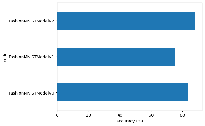
Using the Model
Alright, we’ve compared our models to each other, let’s further evaluate our best performing model, model_2.
Source
def make_predictions(model: torch.nn.Module, data: list, device: torch.device = device):
    pred_probs = []
    model.eval()
    with torch.inference_mode():
        for sample in data:
            # Prepare sample
            sample = torch.unsqueeze(sample, dim=0).to(device) # Add an extra dimension and send sample to device

            # Forward pass (model outputs raw logit)
            pred_logit = model(sample)

            # Get prediction probability (logit -> prediction probability)
            pred_prob = torch.softmax(pred_logit.squeeze(), dim=0) # note: perform softmax on the "logits" dimension, not "batch" dimension (in this case we have a batch size of 1, so can perform on dim=0)

            # Get pred_prob off GPU for further calculations
            pred_probs.append(pred_prob.cpu())

    # Stack the pred_probs to turn list into a tensor
    return torch.stack(pred_probs)
import random
random.seed(42)
test_samples = []
test_labels = []
for sample, label in random.sample(list(test_data), k=9):
test_samples.append(sample)
test_labels.append(label)
# View the first test sample shape and label
print(f"Test sample image shape: {test_samples[0].shape}\nTest sample label: {test_labels[0]} ({class_names[test_labels[0]]})")Test sample image shape: torch.Size([1, 28, 28])
Test sample label: 5 (Sandal)
And now we can use our make_predictions() function to predict on test_samples.
# Make predictions on test samples with model 2
pred_probs= make_predictions(model=model_2,
                             data=test_samples)

# View first two prediction probabilities list
pred_probs[:2]
tensor([[2.1741e-07, 6.4996e-08, 6.2809e-08, 6.1916e-07, 1.4296e-08, 9.9988e-01,
2.1959e-07, 8.9872e-06, 2.2469e-05, 8.3665e-05],
[2.4364e-02, 6.4675e-01, 1.8973e-03, 6.7734e-02, 8.7493e-02, 6.1955e-04,
1.7022e-01, 2.3094e-04, 1.1909e-04, 5.6674e-04]])And now we can go from prediction probabilities to prediction labels by taking the torch.argmax() of the output of the torch.softmax() activation function.
# Turn the prediction probabilities into prediction labels by taking the argmax()
pred_classes = pred_probs.argmax(dim=1)
pred_classes
tensor([5, 1, 7, 4, 3, 0, 4, 7, 1])# Are our predictions in the same form as our test labels?
test_labels, pred_classes([5, 1, 7, 4, 3, 0, 4, 7, 1], tensor([5, 1, 7, 4, 3, 0, 4, 7, 1]))Now our predicted classes are in the same format as our test labels, we can compare.
Since we’re dealing with image data, let’s try to visualize the data!
# Plot predictions
plt.figure(figsize=(9, 9))
nrows = 3
ncols = 3
for i, sample in enumerate(test_samples):
  # Create a subplot
  plt.subplot(nrows, ncols, i+1)

  # Plot the target image
  plt.imshow(sample.squeeze(), cmap="gray")

  # Find the prediction label (in text form, e.g. "Sandal")
  pred_label = class_names[pred_classes[i]]

  # Get the truth label (in text form, e.g. "T-shirt")
  truth_label = class_names[test_labels[i]]

  # Create the title text of the plot
  title_text = f"Pred: {pred_label} | Truth: {truth_label}"

  # Check for equality and change title colour accordingly
  if pred_label == truth_label:
      plt.title(title_text, fontsize=10, c="g") # green text if correct
  else:
      plt.title(title_text, fontsize=10, c="r") # red text if wrong
  plt.axis(False);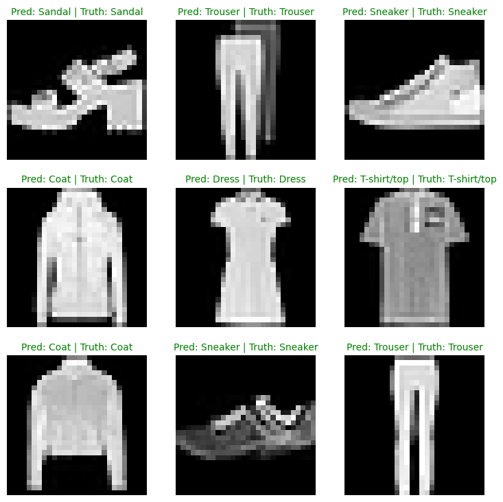
Pretty good! Especially given the simplicity of the model, we got some solid results!
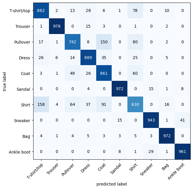
Confusion Matrix
There are many different evaluation metrics we can use for classification problems. We’ll be using the Confusion Matrix.
A confusion matrix shows you where your classification model got confused between predictions and true labels.
Make predictions with our trained model,
model_2(a confusion matrix compares predictions to true labels).Make a confusion matrix using
torchmetrics.ConfusionMatrix.Plot the confusion matrix using
mlxtend.plotting.plot_confusion_matrix().
Let’s start by making predictions with our trained model.
# Import tqdm for progress bar
from tqdm.auto import tqdm

# 1. Make predictions with trained model
y_preds = []
model_2.eval()
with torch.inference_mode():
  for X, y in tqdm(test_dataloader, desc="Making predictions"):
    # Send data and targets to target device
    X, y = X.to('cpu'), y.to('cpu')
    # Do the forward pass
    y_logit = model_2(X)
    # Turn predictions from logits -> prediction probabilities -> predictions labels
    y_pred = torch.softmax(y_logit, dim=1).argmax(dim=1) # note: perform softmax on the "logits" dimension, not "batch" dimension (in this case we have a batch size of 32, so can perform on dim=1)
    # Put predictions on CPU for evaluation
    y_preds.append(y_pred.cpu())
# Concatenate list of predictions into a tensor
y_pred_tensor = torch.cat(y_preds)
Making predictions: 100%|██████████| 313/313 [00:01<00:00, 225.81it/s]
from torchmetrics import ConfusionMatrix
from mlxtend.plotting import plot_confusion_matrix

# 2. Setup confusion matrix instance and compare predictions to targets
confmat = ConfusionMatrix(num_classes=len(class_names), task='multiclass')
confmat_tensor = confmat(preds=y_pred_tensor,
                         target=test_data.targets)

# 3. Plot the confusion matrix
fig, ax = plot_confusion_matrix(
    conf_mat=confmat_tensor.numpy(), # matplotlib likes working with NumPy
    class_names=class_names, # turn the row and column labels into class names
    figsize=(10, 7)
);
For some popular vision models check out timm (Torch Image Models)
For a more in depth version of today’s material watch MIT’s Introduction to Deep Computer Vision lecture.