Assignment 4: Taxi Classifiers

CSci 39542: Introduction to Data Science¶

Department of Computer Science
Hunter College, City University of New York
Spring 2026

Program Description¶

Due AoE, Tuesday, 5 May.

Learning Objective: to train and validate models, given quantitative and qualitative data, as well as assessing model quality.

Available Libraries: pandas, datetime, pickle, pytest, sklearn.ensemble, sklearn.model_selection, sklearn.metrics, sklearn.svm, and core Python 3.6+. (Note if you use our annonations, you should also import Union.)

Data Sources:2021 Yellow Taxi Trip Data and NYC Taxi Zones from OpenData NYC.

Sample Datasets: taxi_new_years_day_2021.csv, taxi_4July2021.csv, taxi_jfk_june2021.csv, and taxi_zones.csv.

This program is tailored to the NYC OpenData Yellow Taxi Trip Data and follows standard strategy for data cleaning and model building:

1. Read in datasets, merging and cleaning as needed.

2. Impute missing values (we will use median for the ordinal values and “most popular” for nominal values).

3. Use categorical encoding for qualitative values.

4. Split our dataset into training and testing sets.

5. Fit a model, or multiple models, to the training dataset.

6. Validate the models using the testing dataset.

7. Develop test suites, using pytest, to ensure that correctness of your code.

To identify which trips are most likely to cross between boroughs, this program will focus on building several classifiers on both the categorical and numerical features of our dataset.

NYC OpenData Yellow Taxi Trip Data¶

This program uses two datasets from NYC Open Data:

• 2021 Yellow Taxi Trip Data and

• NYC Taxi Zones.

See Proram 1 for directions on how to download datasets from NYC Open Data. The sample datasets are filtered, before downloading, by pickup time tpep_pickup_datetime and pickup location PULocationID. Create a practice dataset from your birthday or favorite day in 2021 to use to test your code.

`

Preparing Data¶

Once you have downloaded some test data sets to your device, the next thing to do is format the data to be usable for analysis. We will need to do some cleaning, as well as imputing missing values and encoding categorical values. Once we have the cleaned the data, we can split it into training and testing data sets. Add the following functions to your Python program:

• import_data(file_name) -> pd.DataFrame: This function takes as one input parameter:

  • file_name: the name of a CSV file containing 2021 Yellow Taxi Trip Data from OpenData NYC.

  The data in the file is read into a DataFrame, restricted to the columns:

  VendorID,tpep_pickup_datetime,tpep_dropoff_datetime,passenger_count,trip_distance,PULocationID,DOLocationID,fare_amount,tip_amount,tolls_amount,total_amount

  Any rows where the total_amount is 0 or negative or trip_distance is larger than 200 are dropped. The resulting DataFrame is returned.

• add_tip_time_features(df) -> pd.DataFrame: This function takes one input:

  • df: a DataFrame containing 2021 Yellow Taxi Trip Data from OpenData NYC.

  The function computes 3 new columns:

  • percent_tip: which is 100*tip_amount/(total_amount-tip_amount)

  • duration: the time the trip took in minutes.

  • dayofweek: the day of the week that the trip started, represented as 0 for Monday, 1 for Tuesday, ... 6 for Sunday.

  The original DataFrame with these additional three columns is returned.
  Hint: See Chapter 9.4 for transforming strings to datetime objects.

• impute_numeric_cols(df, x_num_cols) -> pd.DataFrame: This function takes two inputs:

  • df: a DataFrame containing Yellow Taxi Trip Data from OpenData NYC.

  • x_num_cols: a list of numerical columns in df.

  Missing data in the columns x_num_cols are replaced with the median of the column.
  Returns the resulting DataFrame.

• add_boro(df, file_name) -> pd.DataFrame: This function takes as two input parameters:

  • df: a DataFrame containing 2021 Yellow Taxi Trip Data from OpenData NYC.

  • file_name: the name of a CSV file containing NYC Taxi Zones from OpenData NYC.

  Makes a DataFrame, using file_name, to add pick up and drop off boroughs to df. In particular, adds two new columns to the df:

  • PU_borough that contain the borough corresponding to the pick up taxi zone ID (stored in PULocationID), and

  • DO_borough that contain the borough corresponding to the drop off taxi zone (stored in DOLocationID)

  Returns df with these two additional columns (PU_borough and DO_borough).

• add_flags(df) -> pd.DataFrame: This function takes one input parameter:

  • df: a DataFrame containing 2021 Yellow Taxi Trip Data from OpenData NYC to which add_boro() has been applied.

  Adds two new columns:

  • paid_toll which is 1 if a toll was paid on the trip and 0 in no tolls were paid.

  • cross_boro which is 1 if the trip started and ended in different borough, and 0 if the trip started and ended in the same borough.

  Returns df with these two additional columns (paid_toll and cross_boro).

• encode_categorical_col(col,prefix) -> pd.DataFrame: This function takes two input parameters:

  • col: a column of categorical data.

  • prefix: a prefix to use for the labels of the resulting columns.

  Takes a column of categorical data and uses categorical encoding to create a new DataFrame with the k-1 columns, where k is the number of different nomial values for the column. Your function should create k columns, one for each value, labels by the prefix concatenated with the value. The columns should be sorted and the DataFrame restricted to the first k-1 columns returned. For example, if the column contains values: ‘Bronx’, ‘Brooklyn’, ‘Manhattan’, ‘Queens’, and ‘Staten Island’, and the prefix parameter has the value ‘PU_’ (and set the separators to be the empty string: prefix_sep=''), then the resulting columns would be labeled: ‘PU_Bronx’, ‘PU_Brooklyn’, ‘PU_Manhattan’, ‘PU_Queens’, and ‘PU_Staten Island’. The last one alphabetically is dropped (in this example, ‘PU_Staten Island’) and the DataFrame restricted to the first k-1 columns is returned.

• split_test_train(df, xes_col_names, y_col_name, test_size=0.25, random_state=2023) -> Union[pd.DataFrame, pd.DataFrame, pd.Series(), pd.Series()]: This function takes 5 input parameters:

  • df: a DataFrame containing 2021 Yellow Taxi Trip Data from OpenData NYC to which add_boro() has been applied.

  • y_col_name: the name of the column of the dependent variable.

  • xes_col_names: a list of columns that contain the independent variables.

  • test_size: accepts a float between 0 and 1 and represents the proportion of the data set to use for training. This parameter has a default value of 0.25.

  • random_state: Used as a seed to the randomization. This parameter has a default value of 2023.

  Calls sklearn’s train_test_split function to split the data set into a training and testing subsets and returns: x_train, x_test, y_train, y_test.

  Hint: see the examples from Lectures for a similar splitting of data into training and testing datasets.

For example, let’s start by setting up a DataFrame, with the file, taxi_4July2021.csv, add in the tip and time features, and imputing missing values for passenger_count:

which prints:

Next, let’s use our new functions to impute passenger counts and add in boroughs for the pick up and drop off locations:

which prints out the new columns:

We can add the indicators for if a toll was paid and if the trip started and ended in different boroughs:

prints:

Let’s explore the data some:

The resulting plots are:

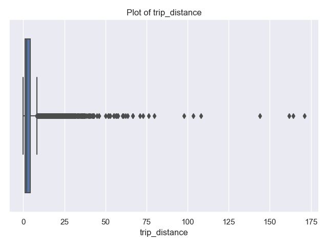
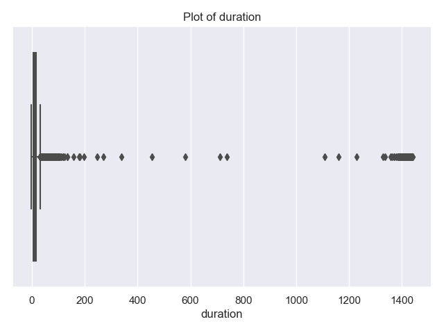
and show that most trips are short in distance and time. There’s a some long trips and very long durations. The latter are likely measurement errors (e.g. mistakenly not ending the trip on the trip recorder), since it’s unlikely that there are many trips of 240 minutes (4 hours) or more.

Let’s look at the trips of over 4 hours and also those of more than 100 miles:

The farthest traveled of the 157 trips that took more than 4 hours is just under 19.86. This seems much more likely an error in the recording device than actual trips. Let’s look at the long trips:

To focus on trips that stay within the city, let’s limit our data to trips that are less than 50 miles in distance, as well as less than 4 hours in duration. And, explore the data by making scatter plots of some of the features:

As discussed in Chapter 24, we added jitter to the y-values to better visualize the data since so much has similar values:

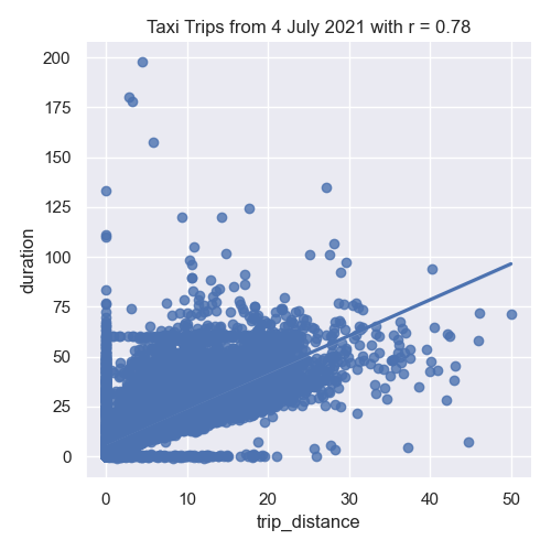
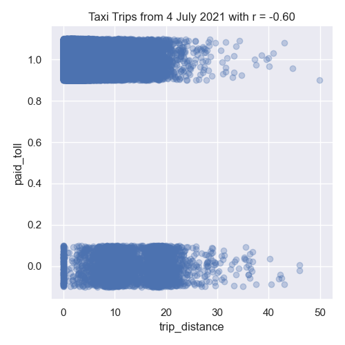
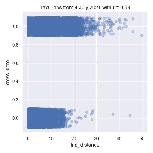
In our left image, the distance traveled and the duration of the trip are strongly correlated. The middle image show negative correlation between trip distance and paying tolls. While the right images shows the trip distance positively correlated with trips that start and end in different boroughs.

Next, let’s encode the categorical columns for pick up and drop off boroughs so we can use them as inputs for our model.

Let’s combine all the DataFrames into one (using concat along column axis):

For the taxi data, there is a special zone for trips to Newark Airport, and as such we have a drop off borough location of 'DO_EWR'. We’ll focus on the numeric columns, split our data into training and testing data sets:

Building Classifers¶

In Lectures 10, 11 and 12 , we introduced models for classifying data. We will use three of those classifiers here: logistic regression, support vector machine classifier (SVC), and random forests. All are implemented in scikit-learn and we will

• fit_logistic_regression(x_train, y_train,penalty=None,max_iter=1000,random_state=2023) -> object: This function takes five input parameter:

  • x_train: the indepenent variable(s) for the analysis.

  • y_train: the dependent variable for the analysis.

  • penalty: the type of regularization applied. The default value for this parameter is None.

  • max_iter: number of iterations allowed when fitting model. The default value for this parameter is 1000.

  • random_state: Used as a seed to the randomization. This parameter has a default value of 2023.

  Fits a logistic regression model to the x_train and y_train data, using the logistic model from sklearn.linear_model. The model should use the solver = 'saga' to allow all the options for regularization (called penalty as the option to the model) be any of 'elasticnet', 'l1', 'l2', and 'none'). The parameter max_iter should also be used when fitting the model. The resulting model should be returned as bytestream, using pickle.

• fit_svc(x_train, y_train,kernel='none',max_iter=1000,random_state=2023) -> object: This function takes five input parameter:

  • x_train: the indepenent variable(s) for the analysis.

  • y_train: the dependent variable for the analysis.

  • kernel: the type of kernel used. The default value for this parameter is ‘rbf’.

  • max_iter: number of iterations allowed when fitting model. The default value for this parameter is 1000.

  • random_state: Used as a seed to the randomization. This parameter has a default value of 2023.

  Fits a support vector machine classifier model to the x_train and y_train data, using the logistic model from sklearn.svm. The model should use the kernel speficied and can be any of the following 'linear', 'poly', 'rbf', and 'sigmoid'). The parameter max_iter should also be used when fitting the model. The resulting model should be returned as bytestream, using pickle.

• fit_random_forest(x_train, y_train,num_trees=100,random_state=2023) -> object: This function takes four input parameter:

  • x_train: the indepenent variable(s) for the analysis.

  • y_train: the dependent variable for the analysis.

  • num_trees: the number of decision trees in the forest classifier. The default value for this parameter is 100.

  • random_state: Used as a seed to the randomization. This parameter has a default value of 2023.

  Fits a random forest model to the x_train and y_train data, using the logistic model from sklearn.ensemble. The parameter num_trees should also be used when fitting the model as the number of estimators, or trees in the forest. The resulting model should be returned as bytestream, using pickle.

We’ll use these functions to build a list of models (as serialized objects) for later use. We’ll try first just a single independent variable, trip_distance, and build a classifiers to predict when trips start in one borough and end in another (when cross_boro is 1). Since some classifiers expect data to be in standard units (introduced in lecture and Program 2), we first put the training sets in standard units and transform the testing sets to be in the same units:

For each type of classifier, we will set up a model for the different parameters available:

    Fitting a logistic model with None regularization.
    Fitting a logistic model with l1 regularization.
    Fitting a logistic model with l2 regularization.
    Fitting a random forest model with 10 number of trees.
    Fitting a random forest model with 100 number of trees.
    Fitting a random forest model with 1000 number of trees.
    Fitting a SVC with linear kernel.
    Fitting a SVC with poly kernel.
    /Users/stjohn/opt/anaconda3/lib/python3.8/site-packages/sklearn/svm/_base.py:299: ConvergenceWarning: Solver terminated early (max_iter=50000).  Consider pre-processing your data with StandardScaler or MinMaxScaler.
      warnings.warn(
    Fitting a SVC with rbf kernel.
    Fitting a SVC with sigmoid kernel....)

Evaluating Our Classifiers¶

We have build a list of multiple classifiers and now will evaluate how well each works on the training data as well as the data we saved for testing.

• predict_using_trained_model(mod_pkl, xes, yes) -> Union[float, float]: This function takes three inputs:

  • mod_pkl: a trained model for the data, stored in pickle format.

  • xes: an array or DataFrame of numeric columns with no null values.

  • yes: an array or DataFrame of numeric columns with no null values.

  Computes and returns the mean squared error and r2 score between the values predicted by the model (mod on x) and the actual values (y). Note that sklearn.metrics contains two functions that may be of use: mean_squared_error and r2_score.

• best_fit(mod_list, name_list, xes, yes, verbose=False) -> Union[object, str]: This function takes five inputs:

  • mod_list: a list of trained models for the data, each stored in pickle format.

  • name_list: a list of trained models for the data, each stored in pickle format.

  • xes: an array or DataFrame of numeric columns with no null values.

  • yes: an array or DataFrame of numeric columns with no null values. verbose: when True, prints out the MSE cost for each model tried (in format: f'MSE cost for model {mod_name} poly model: {error:.3f}' for each mod_name in name_list. It has a default value of False.

  For each model in mod_list, computes the r2 score between the values predicted by the model (mod on x) and the actual values (y), and returns the pickled model and its name.

Let’s run the logistic models we build above:

print(f'For independent variables:  {x_cols}:')
for mod,name in zip(mod_list[:3],name_list[:3]):
    print(f'For model {name}:')
    mse_tr, r2_tr = predict_using_trained_model(mod,x_tr_std,y_train)
    print(f'\ttraining data: mean squared error = {mse_tr:8.8} and r2 = {r2_tr:4.4}.')
    mse_val, r2_val = predict_using_trained_model(mod,x_te_std,y_test)
    print(f'\ttesting data: mean squared error = {mse_val:8.8} and r2 = {r2_val:4.4}.')

which prints:

For independent variables:  ['trip_distance', 'dayofweek', 'paid_toll', 'PU_Bronx', 'PU_Brooklyn', 'PU_Manhattan', 'PU_Queens']:
For model logistic regression with None regularization:
        training data: mean squared error = 0.070102269 and r2 = 0.5002.
        testing data: mean squared error = 0.06801544 and r2 = 0.4981.
For model logistic regression with l1 regularization:
        training data: mean squared error = 0.070124454 and r2 =  0.5.
        testing data: mean squared error = 0.06801544 and r2 = 0.4981.
For model logistic regression with l2 regularization:
        training data: mean squared error = 0.070124454 and r2 =  0.5.
        testing data: mean squared error = 0.06801544 and r2 = 0.4981.

All of the models do better with the training subset than the testing subset. Let’s look at which model did best of all considered:

print(f'For independent variables:  {x_cols}:')
for mod,name in zip(pkl_models[:3],mod_names[:3]):
    print(f'For model {name}:')
    mse_tr, r2_tr = predict_using_trained_model(mod,x_tr_std,y_train)
    print(f'\ttraining data: mean squared error = {mse_tr:8.8} and r2 = {r2_tr:4.4}.')
    mse_val, r2_val = predict_using_trained_model(mod,x_te_std,y_test)
    print(f'\ttesting data: mean squared error = {mse_val:8.8} and r2 = {r2_val:4.4}.')
best_mod, best_name = best_fit(pkl_models,mod_names, x_te_std, y_test, verbose=True)
print(f'The best mode is {best_name}.')    

since we had the verbose flag on, we can see the computations:

MSE cost for model logistic regression with l1 regularization poly model: 0.068
MSE cost for model logistic regression with l2 regularization poly model: 0.068
MSE cost for model random forest with 10 number of trees poly model: 0.076
MSE cost for model random forest with 100 number of trees poly model: 0.075
MSE cost for model random forest with 1000 number of trees poly model: 0.076
MSE cost for model SVC with linear kernel poly model: 0.070
MSE cost for model SVC with poly kernel poly model: 0.075
MSE cost for model SVC with rbf kernel poly model: 0.067
MSE cost for model SVC with sigmoid kernel poly model: 0.131
The best mode is SVC with rbf kernel.

Test Suites¶

In Program 3, we introduced pytest. In addition to the assert statements used, we will also use parametrizations for this program. The basic format is:

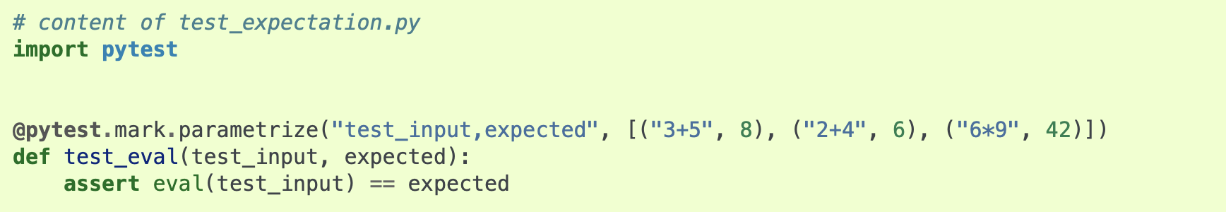
The parametrize list allows you to specify the inputs and expected outputs for the function you are testing. You can define

• test_impute_numeric_cols(test_df,test_cols,expected): This function takes three inputs, provided by the parametriziations:

  • test_df: A DataFrame containing the test_cols.

  • test_cols: A list of columns for the DataFrame test_df.

  • expected: A DataFrame containing the expected output for the inpute_numeric_cols(test_df,test_cols).

  This test function uses pytest to test the impute_numeric_cols() function. It assert True if impute_numeric_cols() is correct and False otherwise.

• test_add_flags(test_df,expected): This function takes two inputs, provided by the parametriziations:

  • test_df: A DataFrame containing the columns expected for the add_flags() function.

  • expected: A DataFrame containing the expected output for the add_flags(test_df).

  This test function uses pytest to test the add_flags() function. It assert True if add_flags() is correct and False otherwise.

Preceding each of these test functions, you should include @pytest.mark.parametrize list. For example, the first testing function should be of the format:

test_data = [ """TRIPLES OF DATA TO TEST GOES HERE""" ]
@pytest.mark.parametrize("test_df,test_cols,expected", test_data)
def test_impute_numeric_cols(test_df,test_cols,expected):
    assert test_impute_numeric_cols(test_df,test_cols).equals(expected)

Hints:

• You can run pytest locally from the command line. To see only errors and results, use the disable-warnings flag:

  pytest --disable-warnings p4.py 

• When comparing DataFrames, you may find the equals() method helpful.